Geometry & Recognition

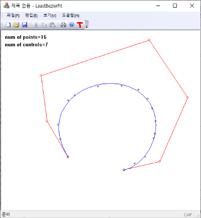
$$ \{ {\bf C}_k \} =\text{argmin}(L) \\ L = \sum_{k=0}^{N-1} \left|  {\bf P}_k - \sum_{i=0}^n  b_{i,n} (t_k ) {\bf C} _i   \right|^2 $$

\begin{gather} t_k = d_k / d_{N-1}, \quad d_k = d_{k-1} + | {\bf P}_k -{\bf P}_{k-1}|\end{gather}

$$\text{Bernstein basis polynomial: } b_{i, n} (t)= \begin{pmatrix} n \\i \end{pmatrix} t^{i} (1-t)^{n-i} = \sum_{j=0}^n t^j  M_{ji} $$

$$ M_{ji} = \frac{n!}{(n-j)!} \frac{ (-1)^{j+i}}{ i! (j-i)!} =(-1)^{j+i}  M_{jj} \begin{pmatrix} j\\i  \end{pmatrix} \quad (j\ge i)$$

$$ \text{note: }~M_{jj} = \begin{pmatrix} n\\j \end{pmatrix},\qquad M_{ji}=0\quad (j<i)$$

// calculate binomial coefficients using Pascal's triangle
void binomialCoeffs(int n, double** C) {
    // binomial coefficients
    for (int i = 0; i <= n; i++)
        for (int j = 0; j <= i; j++)
            if (j == 0 || j == i) C[i][j] = 1;
            else                  C[i][j] = C[i - 1][j - 1] + C[i - 1][j];
}
void basisMatrix(int degree, std::vector<double>& M) {
    const int n = degree + 1;
    double **C = new double* [n];
    C[0] = new double [n * n];
    for (int i = 1; i < n; i++) 
        C[i] = C[i-1] + n;
    // C[degree, k]; k=0,..,degree)
    binomialCoeffs(degree, C);
    // seting the diagonal;
    M.resize(n * n, 0); // lower triangle; 
    for (int j = 0; j <= degree; j++)
        M[j * n + j] = C[degree][j];
    // compute the remainings;
    for (int i = 0; i <= degree; i++) 
        for (int j = i + 1; j <= degree; j++)
            M[j * n + i] = ((j + i) & 1 ? -1 : 1) * C[j][i] * M[j * n + j];
    
    delete [] C[0]; delete [] C;
}

주어진 데이터를 잘 피팅하는 직선을 찾기 위해서는 데이터를 이루는 각 점의 $y$ 값과 같은 위치에서 구하려는 직선과의 차이 (residual)의 제곱을 최소화시키는 조건을 사용한다. 그러나 직선의 기울기가 매우 커지는 경우에는  데이터에 들어있는 outlier에 대해서는 그 차이가 매우 커지는 경우가 발생할 수도 있어 올바른 피팅을 방해할 수 있다. 이를 수정하는 간단한 방법 중 하나는 $y$값의 차이를 이용하지 않고 데이터와 직선 간의 최단거리를 이용하는 것이다. 

수평에서 기울어진 각도가 $\theta$이고 원점에서 거리가 $s$인 직선의 방정식은 

$$ x \sin \theta - y \cos \theta + s=0$$

이고, 한 점 $(x_i, y_i)$에서 이 직선까지 거리는

$$ d_i = | \sin \theta y_i - \cos \theta x_i + s|$$

이다. 따라서 주어진 데이터에서 떨어진 거리 제곱의 합이 최소인 직선을 구하기 위해서는 다음을 최소화시키는 $\theta, s$을 구해야 한다. $$ L = \sum_i \big( \sin \theta x_i - \cos \theta y_i +s \big)^2 \\ (\theta, s)=\text{argmin}(L)$$

$\theta$와 $s$에 대한 극값 조건에서 

$$\frac{1}{2} \frac{\partial L}{\partial \theta} = \frac{1}{2} \sin 2 \theta \sum_i (x_i^2 - y_i^2) - \cos 2 \theta \sum x_i y_i + s \sin \theta \sum_i x_i + s \cos \theta \sum_i y_i = 0$$

$$ \frac{1}{2}\frac{\partial L}{\partial s}=\cos \theta \sum y_i  - \sin \theta \sum_i x_i - N s=0$$

주어진 데이터의 질량중심계에서 계산을 수행하면 $\sum_i x_i = \sum_i y_i =0$ 이므로 데이터의 2차 모멘트를 $$ A= \sum_i (x_i^2 - y_i^2), \qquad B = \sum_i x_i y_i $$로 놓으면 직선의 파라미터를 결정하는 식은

$$ \frac{1}{2} A \sin 2 \theta   - B \cos 2 \theta = 0  \qquad \to \quad  \tan 2\theta = \frac{2B}{A} \\ s = 0$$

두 번째 식은 직선이 질량중심(질량중심계에서 원점)을 통과함을 의미한다. 첫번째 식을 풀면

$$ \tan \theta = \frac{- A \pm \sqrt{A^2 + (2B)^2 }}{2B}$$

두 해 중에서 극소값 조건을 만족시키는 해가 직선을 결정한다. 그런데

$$ \frac{1}{2}\frac{\partial^2 L}{\partial \theta^2}=  A \cos 2 \theta + 2B \sin 2 \theta = \pm \sqrt{A^2 + (2B)^2}  >0$$

이므로 위쪽 부호로 직선($x\sin \theta = y\cos \theta$)이 정해진다. 질량중심계에서는 원점을 지나지만 원좌표계로 돌아오면 데이터의 질량중심을 통과하도록 평행이동시키면 된다.

$$  \left(-A+ \sqrt{A^2+ (2B)^2} \right)  (x-\bar{x}) = 2B (y - \bar{y})  $$

여기서 주어진 데이터의 질량중심은 원좌표계에서

$$ \bar{x} = \frac{1}{N} \sum_i x_i, \quad \bar{y} = \frac{1}{N} \sum_i y_i$$

이다. 또한 원좌표계에서 $A$와 $B$의 계산은 

$$ A = \sum_i [ (x_i - \bar{x})^2 - (y_i - \bar{y})^2], \qquad B = \sum (x_i  - \bar{x})(y_i - \bar{y})$$ 

이 결과는 데이터 분포에 PCA를 적용해서 얻은 결과와 동일하다. PCA에서는 공분산 행렬의 고유값이 큰 쪽에 해당하는 고유벡터가 직선의 방향을 결정했다. https://kipl.tistory.com/211.  또한 통계에서는 Deming regression이라고 불린다.

최소 자승법 문제는 추정치와 실제의 측정치와의 차이를 최소로 만드는 parameter vector를 구하는 것이다.
$$\underset{\mathbf{x}} {\text{argmin}} ~|\mathbf{A}. \mathbf{x} - \mathbf{b}|^2.$$

여기서 design matrix $\mathbf{A}$는 추정에 사용이 된 basis 함수를 각각의 독립변수에서 계산한 값이고, $\mathbf{x}$는 구하고자 하는 parameter vector이며, $\mathbf{b}$는 측정값 vector이다. 예를 들면 주어진 측정값을 $n-1$차의 다항식을 이용하여서 피팅하려고 하는 경우에는 parameter는 다항식의 계수가 되며 $n$-차원의 vector space을 형성하게 되며, $\mathbf{A}$는

$$   A_{ij} = (x_i)^j ,  \quad j=0,..., n-1$$

가 일 것이다. 일반적으로 $A_{ij}$는 $x_i$에서 계산된 basis-함수의 값이 된다. 위의 식을 $\mathbf{x}$에 대해서 미분을 하면 극값을 취하면 최소자승 문제는 아래의 행렬식을 푸는 문제가 된다

$$    (\mathbf{A}^T. \mathbf{A}) .\mathbf{x} =  \mathbf{A}^T.  \mathbf{b}.$$

$\mathbf{A}^T. \mathbf{A}$ 은 $n\times n$ matrix다. 이 행렬이 역행렬을 가지게 되면

 $$ \mathbf{x} = (\mathbf{A}^T. \mathbf{A})^{-1} . (\mathbf{A}. \mathbf{b}),$$

를 하여서 원하는 parameter vector를 얻을 수 있다. 그러나 피팅 문제에 따라 행렬 $\mathbf{A}^T. \mathbf{A}$가 매우 singular 해져 역행렬을 구할 수 없게 되는 경우에 종종 생긴다. 예를 들면, 저주파의 신호를 고주파 기저 함수를 이용하여서 최소자승법을 사용하고자 하는 경우 등에 이러한 문제에 부딪히게 된다. 이런 경우에는 직접적으로 $\mathbf{A}^T. \mathbf{A}$의 역행렬을 구하는 방법을 이용할 수 없고

$$   \mathbf{A} .\mathbf{x} =  \mathbf{b}$$

의 식을 $\mathbf{A}$의 SVD(Singular Value Decomposition)를 이용하여서 풀 수가 있다. $\mathbf{A}$를 SVD 하면 $\mathbf{A}_{m\times n}=\mathbf{U}_{m\times n} . \mathbf{w}_{n\times n}. \mathbf{V}_{n\times n}^T $의 형태로 분해할 수 있다. 여기서 $\mathbf{w}=\text{diag}(\underbrace{w_0, w_1,...}_{\text{nonzero}},0,..,0)$로 쓰여지는 대각행렬이다. matrix $\mathbf{U}$와 $\mathbf{V}$의 column vector를 사용하면
$$ \mathbf{A}  =\sum_{w_k \ne 0} w_k \mathbf{u}_k \otimes \mathbf{v}_k^T$$

의 형태로 쓰인다. $\mathbf{u}_k$는 $\mathbf{U}$의 $k$-번째 열벡터이고, $\mathbf{v}_k$는 $\mathbf{V}$의 $k$-번째 열벡터로 각각 orthonormal basis를 형성한다. parameter 벡터를 $\{ \mathbf{v}_k \}$ basis로 전개를 하면 영이 아닌 singularvalue에 해당하는 성분만 가지게 된다. 구체적으로 위의 $\mathbf{A}$ 분해와 $\mathbf{u}_j^T.\mathbf{u}_k=\delta_{jk}$, 그리고 $\sum_k \mathbf{v}_k \otimes \mathbf{v}_k^T= \mathbf{I}_{n\times n}$임을 이용하면,

\begin{gather}  \mathbf{v}_k^T . \mathbf{x} = \mathbf{u}_k^T . \mathbf{b} / w_k, \quad w_k \ne 0, \\                    \mathbf{v}_k^T . \mathbf{x} = 0, \quad w_k = 0, \\  \rightarrow ~~\mathbf{x} = \sum _{w_k \ne 0 } ( \mathbf{u}_k^T . \mathbf{b} / w_k)  \mathbf{ v} _k , \end{gather}

이어서 위의 해를 구할 수 있다. 이 해는 $|\mathbf{A} . \mathbf{x} -  \mathbf{b}|^2$를 최소화한다.

int svd(double *A, int m, int n, double* w, double *V); // from cmath libary.
void fit_func(double x, double val[], int n) {          // polynomial fitting sample;
    val[0] = 1;
    for(int i = 1; i < n; ++i)
        val[i] = x * val[i - 1];
}
#define EPSILON 1.E-8
int svd_fit(const double x[], const double y[], const int m, const int n,
            void (*fit_func)(double , double [], int ),
            double params[],
            double *error)
{
    double *A = new double [m * n];
    double *w = new double [n];
    double *V = new double [n * n];
    // evaluate design matrix;
    for (int i = 0; i < m; ++i)
        fit_func(x[i], &A[i * n + 0], n) ;

    svd(A, m, n, w, V);
    // now A becomes U matrix;
    // truncate small singular values;
    double wmax = 0;
    for (int i = 0; i < n; ++i)
        if (w[i] > wmax) wmax = w[i];
    double thresh = wmax * EPSILON;
    for (int i = 0; i < n; ++i)
        if (w[i] < thresh) w[i] = 0;
    
    // back substitution;
    double *tmp = new double [n];
    for (int j = 0; j < n; ++j) {
        double s = 0;
        if (w[j]) {
            for (int i = 0; i < m; ++i)
                s += A[i * n + j] * y[i];
            s /= w[j];
        }
        tmp[j] = s;
    }
    for (int j = 0; j < n; ++j) {
        double s = 0;
        for (int jj = 0; jj < n; ++jj)
            s += V[j * n + jj] * tmp[jj];
        params[j] = s;
    };

    //estimate error;
    *error = 0;
    for (int i = 0; i < m; ++i) {
        fit_func(x[i], &A[i * n + 0], n); //use A as a tmp buffer;
        double sum = 0;
        for (int j = 0; j < n; ++j) sum += params[j] * A[i * n + j] ;
        double err = (y[i] - sum);
        *error += err * err ;
    }
    delete[] A; delete[] w; delete[] V;
    delete[] tmp;
    return 1;
}

$m$개의 control point $\{\mathbf{Q}_i\}$가 주어지면  $p$차의 B-Spline curve는 basis 함수를 $N_{i, p}(t)$을 써서

$$ \mathbf{B}(t) = \sum_{i=0}^{m-1} N_{i, p}(t) \mathbf{Q}_i $$

로 표현할 수 있다. 이를 이용해서 일정한 순서로 샘플링된 평면상의 $N$개의 입력점 $\{ \mathbf{P}_i \}$을 찾아보자. B-spline 곡선을 이용하면 이 문제는 control 점을 찾는 문제가 된다. 곡선이 입력점을 잘 표현하기 위해서는 곡선과 입력점과의 차이를 최소로 하는 control 점을 찾아야 한다:

$$    \mathbf{ Q}^* = \text{argmin}(L), \quad\quad L:= \sum_{k = 0}^{N-1} | \mathbf{B}(t_k) - \mathbf{P}_k|^2 $$

여기서 $\{ t_k| k=0,1,...,N-1\}$는 입력점이 얻어지는 sample time으로 $0= t_0\le t_1\le...\le t_{N-1}= 1$로 rescale 할 수 있다. 

행렬을 이용해서 식을 좀 더 간결하게 표현할 수 있다. 

$$L = \sum_{k = 0}^{N-1} | \mathbf{B}(t_k) - \mathbf{P}_k|^2 = \sum_{k = 0}^{N-1} \left| \sum_{i=0}^{m-1} N_{i, p}(t_k) \mathbf{Q}_i -  \mathbf{P}_k \right|^2 = \sum_{k = 0}^{N-1} \left| \sum_{i=0}^{m-1} A_{ki} \mathbf{Q}_i - \mathbf{P}_k \right|^2, \\ \quad A_{ki} = N_{i, p}(t_k) $$

로 쓸 수 있으므로, $\hat {Q}= (\mathbf{Q}_0, \mathbf{Q}_1,..., \mathbf{Q}_{m-1})^t$, $\hat {P} = (\mathbf{P}_0, \mathbf{P}_1,..., \mathbf{P}_{N-1})^t$인 벡터, 그리고 $ \hat {A} = (A_{ki})$인 행렬로 보면

$$ L= \left| \hat{A} \cdot \hat {Q} - \hat {P} \right|^2 =  (\hat{Q}^t \cdot \hat {A}^t -\hat{P}^t ) \cdot (\hat{A}\cdot \hat{Q} - \hat{P}).$$

위 식의 값을 최소로 하는 최소자승해는 $\hat {Q}^t$에 대한 미분 값이 0인 벡터를 찾으면 된다; $$ \frac {\partial L}{\partial \hat {Q}^t } = \hat {A}^t \cdot \hat {A} \cdot \hat {Q} - \hat {A}^{t} \cdot \hat {P} = 0.$$ 이 행렬 방정식의 해는

$$ \hat {Q}^* = ( \hat {A} ^t \cdot \hat {A})^{-1} \cdot ( \hat {A}^t \cdot \hat {P})$$ 로 표현된다. $\hat {A} ^t \cdot \hat {A}$가 (banded) real symmetric ($m\times m$) 행렬이므로 Cholesky decomposion을 사용하면 쉽게 해를 구할 수 있다. $\hat{A}$가 banded matrix 형태를 가지는 이유는 basis가 local support에서만 0이 아닌 값을 취하기 때문이다. 

open b-spline(cubic)

int BSplineFit_LS(std::vector<CPoint>& data,
                  int degree,             // cubic(3); 
                  int nc,                 // num of control points;
                  std::vector<double>& X,
                  std::vector<double>& Y) // estimated control points;
{
    // open b-spline;
    std::vector<double> knot((nc - 1) + degree + 2);
    for (int i = 0; i <= nc + degree; i++) knot[i] = i;
    
    std::vector<double> t(data.size());       // parameter;
    double scale = (knot[nc] - knot[degree]) / (data.size()-1);
    for (int i = data.size(); i-->0;) 
        t[i] = knot[degree] + scale * i;

    std::vector<double> A(ndata * nc);
    for (int i = data.size(); i-->0;)
        for (int j = 0; j < nc; j++)
            A[i * nc + j] = Basis(j, degree, &knot[0], t[i]); //A(i,j)=N_j(t_i)

    // S = A^t * A; real-symmetric matrix;
    std::vector<double> Sx(nc * nc);
    std::vector<double> Sy(nc * nc);
    for (int i = 0; i < nc; i++) {
        for (int j = 0; j < nc; j++) {
            double s = 0;
            for (int k = data.size(); k-->0;)
                s += A[k * nc + i] * A[k * nc + j];
            Sx[i * nc + j] = s;
        }
    }
    //copy;
    for (int i = nc*nc; i-->0;) Sy[i] = Sx[i];
    // X = A^t * P.x;  Y = A^t * P.y
    for (int i = 0; i < nc; i++) {
        double sx = 0, sy = 0;
        for (int k = data.size(); k-->0;) {
            sx += A[k * nc + i] * data[k].x;
            sy += A[k * nc + i] * data[k].y;
        };
        X[i] = sx; Y[i] = sy;
    };
    // solve real symmetric linear system; S * x = X, S * y = Y;
    // solvps(S, X) destories the inputs;
    // ccmath-2.2.1 version;
    int res1 = solvps(&Sx[0], &X[0], nc);
    int res2 = solvps(&Sy[0], &Y[0], nc);
    return res1 == 0 && res2 == 0;
};

**네이버 블로그 이전;

점집합을 일반적인 2차 곡선으로 피팅하는 경우에 방정식은

$$ a x^2 + by^2 + cxy +d x + ey +f = 0$$

의 계수를 주어진 데이터를 이용하여서 구해야 한다. 실제 문제에서는 타원, 포물선 쌍곡 선등의 타입에 따라 몇 가지 제약 조건을 넣어 피팅을 한다. 원은 타원의 특별한 경우로 일반적으로 $a = b$, $c = 0$의 제약 조건이 필요하다. 그러나 보다 엄밀하게 제약을 하게 되면 $a = b = 1$의 추가 조건을 줄 수 있다. 이 경우는 점들이 모두 일직선에 있는 경우를 ($a = b = 0$) 취급할 수 없게 된다. 이 예외적인 경우를 제외하고는 최소자승법을 사용하면 계수를 매우 쉽게 구할 수 있기 때문에 많이 이용된다.

문제: 주어진 데이터를 fitting 하는 이차곡선(원)

$$x^2  + y^2 + A x + B  y + C = 0$$

의 계수 $A, B, C$를 최소자승법을 사용해서 구하라. 

주어진 점집합이 원 위의 점이면 우변이 0이 되어야 하나, 실제 데이터를 얻는 과정에서 여러 노이즈에 노출되므로 일반적으로 0이 되지 않는다. 최소자승법은 주어진 점들이 원에서 벗어나는 정도의 제곱 합이 최소가 되도록 하는 계수 $A, B, C$를 결정한다.  원과 점의 편차의 제곱합
$$ L=\sum_ i   \left |x_i^2 + y_i^2 + A x_i + B y_i + C \right|^2 , $$

의 극값을 찾기 위해서 $A, B,$ 그리고 $C$에 대해 미분을 하면

$$\frac{\partial L}{\partial A} = 2 \sum_i (x_i^2 + y_i^2 + A x_i + B y_i + C) x_i = 0, $$

$$\frac{\partial L}{\partial B} = 2 \sum_i (x_i^2 + y_i^2 + A x_i + B y_i + C) y_i = 0, $$

$$\frac{\partial L}{\partial C} = 2 \sum_i (x_i^2 + y_i^2 + A x_i + B y_i + C) = 0. $$

이 연립방정식을 풀면  $A, B, C$를 구할 수 있다. 계산을 단순하게 만들고 수치적 안정성을 높이기 위해 입력점들의 질량중심 

$$ m_x = \frac{1}{N} \sum_i x_i, \quad m_y = \frac{1}{N} \sum_i y_i$$

계에서 계산을 하자. 이를 위해 입력점의 $x$, $y$ 성분에서 각각 $m_x$, $m_y$만큼을 빼준 값을 좌표값으로 대입하면 된다: 

$$ x_i \to x_i - m_x,\quad y_i \to y_i - m_y$$

그러면 질량중심 좌표계에서는 $S_x = \sum_i x_i =0$, $S_y= \sum_i y_i =0$이 된다.

우선 세 번째 식에서 

$$ C = -\frac{S_{x^2} + S_{y^2}}{N} $$

을 얻을 수 있고, 첫번째와 두 번째 식에서는 각각

$$ S_{x^2} A +  S_{xy} B = -  (S_{x^3} + S_{xy^2})  $$

$$ S_{xy}  A  + S_{y^2} B = - (S_{y^3} + S_{x^2 y} )$$

을 얻을 수 있다. 이를 풀면

$$ A = \frac{- S_{y^2} ( S_{x^3} + S_{xy^2}) + S_{xy} (S_{y^3} + S_{x^2y})  }{ S_{x^2} S_{y^2} - S_{xy}^2 } \\ B= \frac{-S_{x^2}(S_{y^3} + S_{x^2 y}) +S_{xy}  (S_{x^3} + S_{xy^2}) }{S_{x^2} S_{y^2}- S_{xy}^2} $$

여기서 주어진 데이터의 각 차수에 해당하는 moment는 아래처럼 계산된다:

추정된 원의 중심 $(c_x, c_y)$는 

$$ c_x = - \frac{A}{2},   \qquad c_y = - \frac{B}{2} $$

로 주어지고, 반지름은 

$$r^2 =  c_x^2 +c_y^2 - C = c_x^2 + c_y^2 + \frac{1}{N}( S_{x^2}+S_{y^2})$$

로 주어진다.

Ref: I. Kasa, A curve fitting procedure and its error analysis. IEEE Trans. Inst. Meas., 25:8-14, 1976

/* 구현 코드: 2024.04.01, typing error 수정 & 질량중심계 계산으로 수정;*/
double circleFit_LS(std::vector<CPoint>& Q, double& cx, double& cy, double& radius) {
    if (Q.size() < 3) return -1;
    double sx2 = 0.0, sy2 = 0.0, sxy  = 0.0;
    double sx3 = 0.0, sy3 = 0.0, sx2y = 0.0, sxy2 = 0.0;
    double mx = 0, my = 0;            /* center of mass;*/
    for (int k = Q.size(); k-->0;)
        mx += Q[k].x, my += Q[k].y;
    mx /= Q.size(); my /= Q.size();
    /* compute moments; */
    for (int k = Q.size(); k-->0;) { /* offset (mx, my)*/
        double x = Q[k].x - mx, xx = x * x;
        double y = Q[k].y - my, yy = y * y;
        sx2  += xx;      sy2  += yy;      sxy  += x * y;
        sx3  += x * xx;  sy3  += y * yy;
        sx2y += xx * y;  sxy2 += yy * x;
    }
    double det = sx2 * sy2 - sxy * sxy;
    if (fabs(det) < 1.e-10) return -1;    /*collinear한 경우임;*/
    /* center in cm frame; */
    double a = sx3 + sxy2;
    double b = sy3 + sx2y;
    cx = (sy2 * a - sxy * b) / det / 2;
    cy = (sx2 * b - sxy * a) / det / 2;
    /* radius squared */
    double radsq = cx * cx + cy * cy + (sx2 + sy2) / Q.size();
    radius = sqrt(radsq);
    cx += mx; cy += my; /* recover offset; */
    return fitError(Q, cx, cy, radius);
}