주어진 영상이 어떤 특정한 물체를 담고 있는지를 알아보려면, 그 물체의 template을 만들어서 영상 위에 겹친 후 픽셀 단위로 순차적으로 이동시키면서 일치하는가를 체크하면 된다. 일치의 여부는 보통의 경우 템플레이트와 영상의 상관계수를 측정하면 된다. 대상 영상이 이진 영상인 경우에는 distance map을 이용하면 좀 더 쉽게 매칭 문제를 해결할 수 있다. 에지 영상을 사용해서 만든 distance map은 이미지 영역의 한 지점에서 가장 가까이에 있는 에지 위치까지의 거리를 알려준다. 매칭하고자 template의 이진 영상을 담고 있는 이미지를 distance map에서 픽셀 단위로 차례로 옮기면서 template 위치에서 distance map이 알려주는 에지까지의 거리 합을 기록하면 총거리의 합이 가장 작은 지점에서 template와 가장 잘 맞는 형상을 찾을 수 있을 것이다.
이 메칭 기법(Chamfer Match)은 모델과 이미지가 서로 회전되어 있지 않아야 하고, 스케일 변형도 없는 경우에 좋은 결과를 얻는다. 스케일 변화가 있는 경우에는 스케일 공간에서 순차적으로 찾는 방법을 쓰면 된다. 모델 영상에 변화가 있는 경우에는 민감하게 반응하므로, 각각의 변화된 모델 영상을 따로 준비하여서 매칭 과정을 수행해야 한다. distance map만 구해지면 매칭 과정이 매우 단순하기 때문에 매칭 비용도 매우 저렴하다. 그리고 거리 값을 적당한 범위에 truncate 하는 것이 보다 robust 한 결과를 준다.
* procedure:
- 입력영상의 에지영상을 구함.
- 입력영상의 에지영상의 distance map을 구함.
- 매칭과정을 실행.

int GetAddressTable(BYTE *subImg, int w, int h, int stride/*=원본이미지 폭*/, int addr[]);
//계산을 보다 빠르게 하기 위해서 subimg에서 template 위치를(distimg에 놓인 경우) 미리 계산함.
int GetAddressTable(BYTE *subImg, int w, int h, int stride/*=원본이미지 폭*/, int addr[]) {
    for(int y=0, k=0; y<h; y++) {
        for(int x=0; x<w; x++){
            if(subImg[y*w+x])
                addr[k++]= y*stride + x ; //template가 dist이미지에서움직일 때 픽셀위치(상대적);
        }
    }
    return (k);    //# of template pixels<= w*h;
}
Matching code;
void ChamferMatch(float* distImg, int w1, int h1, //distance-map;
BYTE* subImg, int w2, int h2, //template-map;
float *match/*[w1 * h1]*/) { //match_score-map(filled with FLT_MAX)
int umax = w1 - w2;
int vmax = h1 - h2;
int uc = w2 / 2; //center_x of template-map;
int vc = h2 / 2; //center_y of template-map;
int *addr = new int [w2 * h2]; //max;
int n = GetAddressTable(subImg, w2, h2, w1, addr) ;
for (int v = 0; v <= vmax; v += 2){ //to speed-up;
for (int u = 0; u <= umax; u += 2){ //to speed-up;
double score=0;
#if (0)
for (int v1 = v, v2 = 0; v1 < h1 && v2 < h2; v1++, v2++){
int i1 = v1 * w1;
int i2 = v2 * w2;
for (int u1 = u, u2 = 0; u1 < w1 && u2 < w2; u1++, u2++) {
if (subImg[i2 + u2])
score += distImg[i1 + u1]; // truncate [0, th_dist];
}
}
#else
int offset = v * w1 + u; //start address;
int i = n;
while(i--) score += distImg[addr[i] + offset];
#endif
//at the center of subimg;
match[(uc + u) + (vc + v) * w1] = score;
}
}
delete[] addr ;
};
입력영상의 에지영상(모델이미지를 포함, 에지를 1픽셀로 조절하지 않았음)

모델영상:
distance map에서 찾은 위치에 template를 오버랩함;


'Image Recognition' 카테고리의 다른 글
| Rolling Ball Transformation (1) | 2008.08.09 |
|---|---|
| Mean Shift Filter (5) | 2008.08.06 |
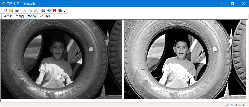
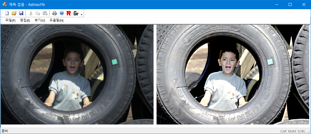
| Retinex Algorithm (2) | 2008.07.26 |
| RANSAC: Circle Fit (0) | 2008.07.21 |
| KMeans Algorithm (0) | 2008.07.19 |