1. Derivative Based Algorithms:
- Thresholded absolute gradient: $$ f =\sum_x \sum _y |I (x+1, y) - I(x, y)| $$ where $|I(x+1, y) - I(x, y)| > \text{threshold};$
- Squared gradient: $$f=\sum_x \sum_y ( I(x+1, y)- I(x, y)) ^2 $$ where $(I(x+1, y) - I(x, y))^2 > \text{threshold};$
- Brenner gradient: $$f=\sum_x \sum_y ( I(x+2, y)- I(x, y)) ^2 $$ where $(I(x+2, y) - I(x, y))^2 > \text{threshold};$
- Tenenbaum gradient: $$f = \sum_x \sum_y (\text{SobelX}^2 (x, y)+ \text{SobelY}^2(x,y));$$
- Energy Laplace: $$f = \sum_x \sum_y ( (L * I) (x, y))^2$$ where $$L =\left[\begin{array}{ccc} -1& -4 & -1 \\ -4 & 20 & -4 \\ -1 & -4 & -1 \end{array} \right]$$
- Sum of modified Laplace: $$f = \sum_x \sum_y (\text{LaplaceX}(x, y)| + |\text{LaplaceY}(x, y)|) $$
- Sum of squared Gaussian derivatives $$f = \frac{1}{\text{total pixels}} \sum_x \sum_y ((\text{Gaussian derivative X}(x,y)) ^2 + (\text{Gaussian derivative Y}(x,y))^2 )$$ where $\sigma = d/(2\sqrt{3})$, $d$ = dimension of the smallest feature;
2. Statistical Algorithms:
- Variance Measure ; $$f = \frac{1}{\text{total pixels}}\sum _x \sum _y ( I (x, y) - \overline{I})^2;$$ where $\overline{I}$ is the mean of image.
- Normalized Variance Measure ; $$f = \frac{1}{\text{total pixels}\times \overline{I}} \sum_x \sum_y ( I(x, y)- \overline{I})^2;$$
- Auto-correlation Measure: $$f = \sum_x\sum_y I(x, y) I(x+1, y) - \sum _x \sum_y I(x, y) I(x+2, y);$$
- Standard Deviation-based Correlation: $$f = \sum_x \sum_y I(x, y) I(x+1, y) - \overline{I}^2(x, y)\times \text{total pixels};$$
3. Histogram-based Algorithms:
- Range Algorithm: $$f =\text{max}\{i| \text{histogram}(i)>0\} - \text{min}\{ i| \text{histogram}(i)>0\};$$
- Entropy Algorithm: $$f=-\sum_{i=0}^{255} p(i) \log_{2} p(i)$$ where $p(i)= \text{histogram}(i)/\text{total pixels};$
4. Other Algorithms:
- Threshold Contents: $$f=\sum_x \sum_y I(x, y)$$ where $I(x,y) \ge \text{threshold};$
- Thresholded Pixel Count: $$f=\sum_x\sum_y \theta(\text{threshold}- I(x, y));$$ where $\theta(x)$ is the step-function.
- Image Power: $$f= \sum_{x}\sum_{y} I^2(x, y)$$ where $I(x, y) \ge\text{threshold};$
Ref: Dynamic evaluation of autofocusing for automated microscopic analysis of blood smear and pap smear, J. Microscopy,227, 15(2007).
728x90
'Image Recognition' 카테고리의 다른 글
| Union-Find Connected Component Labeling (0) | 2012.11.01 |
|---|---|
| RANSAC: Ellipse Fitting (1) | 2012.10.07 |
| Statistical Region Merging (2) | 2012.03.25 |
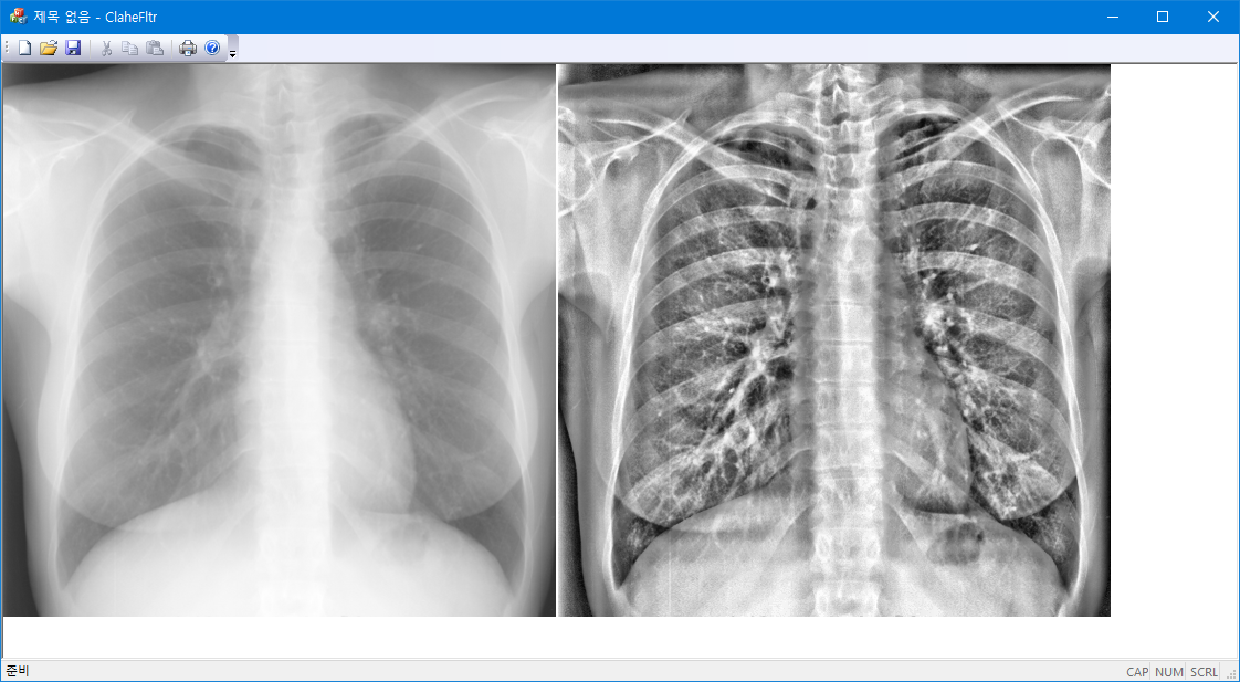
| Local Histogram Equalization (0) | 2012.03.10 |
| 2차원 Savitzky-Golay Filters 응용 (0) | 2012.02.28 |