Otsu 알고리즘은 이미지를 이진화시키는데 기준이 되는 값을 통계적인 방법을 이용해서 결정한다. 같은 클래스(전경/배경)에 속한 픽셀의 그레이 값은 유사한 값을 가져야 하므로 클래스 내에서 픽셀 값의 분산은 되도록이면 작게 나오도록 threshold 값이 결정되어야 한다. 또 잘 분리가 되었다는 것은 클래스 간의 거리가 되도록이면 멀리 떨어져 있다는 의미이므로 클래스 사이의 분산 값은 커야 함을 의미한다. 이 두 가지 요구조건은 동일한 결과를 줌을 수학적으로 보일 수 있다.

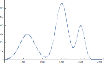
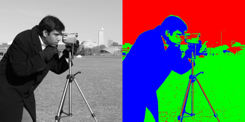
이미지의 이진화는 전경과 배경을 분리하는 작업이므로 클래스의 개수가 2개, 즉, threshold 값이 1개만 필요하다. 그러나 일반적으로 주어진 이미지의 픽셀 값을 임의의 개수의 클래스로 분리할 수도 있다. 아래의 코드는 주어진 이미지의 histogram을 Otsu의 아이디어를 이용해서 nclass개의 클래스로 분리하는 알고리즘을 재귀적으로 구현한 것이다. 영상에서 얻은 히스토그램을 사용하여 도수를 계산할 수 있는 0차 cumulative histogram($\tt ch$)과 평균을 계산할 수 있는 1차 culmuative histogram($\tt cxh$)을 입력으로 사용한다. 

$$ {\tt thresholds}= \text {argmax} \left( \sigma^2_B = \sum_{j=0}^{nclass-1} \omega_j m_j^2 \right)$$


* Otsu 알고리즘을 이용한 이미지 이진화 코드: kipl.tistory.com/17

* 좋은 결과를 얻으려면 히스토그램에 적당한 필터를 적용해서 smooth하게 만드는 과정이 필요하다.

// 0 <= start < n;
double histo_partition(int nclass, double cxh[], int ch[], int n, int start, int th[]) {
    if (nclass < 1) return 0;
    if (nclass == 1) {
        int ws; double ms;
        if (start == 0) {
            ws = ch[n - 1];
            ms = cxh[n - 1] / ws;
        } else {
            ws = ch[n - 1] - ch[start - 1];             // start부터 끝까지 돗수;
            ms = (cxh[n - 1] - cxh[start - 1]) / ws;    // start부터 끝까지 평균값;
        }
        th[0] = n - 1;
        return ws * ms * ms;                            // weighted mean;
    }

    double gain_max = -1;
    int *tt = new int [nclass - 1];
    for (int j = start; j < n; j++) {
        int wj; double mj;
        if (start == 0) {
            wj = ch[j]; 
            mj = cxh[j];                    //mj = cxh[j] / wj;
        }
        else {
            wj = ch[j] - ch[start - 1];     //start부터 j까지 돗수;
            mj = (cxh[j] - cxh[start - 1]); //mj = (cxh[j] - cxh[start - 1]) / wj;
        }
        if (wj == 0) continue;
        mj /= wj;                           //start부터 j까지 평균;
        double gain = wj * mj * mj + histo_partition(nclass - 1, cxh, ch, n, j + 1, tt);
        if (gain > gain_max) {
            th[0] = j;
            for (int k = nclass - 1; k > 0; k--) th[k] = tt[k - 1];
            gain_max = gain;
        }
    }
    delete [] tt;
    return gain_max;
};

trimodal 분포의 분리;

class0: 0~th[0]

class1: (th[0]+1)~th[1],

class2: (th[1]+1)~th[2]=255

th[0]=103, th[1]=172 (th[2]=255)
th[0]=88, th[1]=176, th[2]=255

더보기
// recursive histo-partition 테스트;
// 0--t[0];--t[1];...;--t[nclass-2];t[nclass-1]=255=n-1;
// nclass일 때 threshold 값은 0---(nclss-2)까지;
double GetThreshValues(int hist[], int n, int nclass, int th[]) {
    if (nclass < 1) nclass = 1;
    // preparing for 0-th and 1-th cumulative histograms;
    int *ch = new int [n];          // cdf;
    double *cxh = new double [n];   //1-th cdf;
    ch[0] = hist[0];
    cxh[0] = 0; // = 0 * hist[0]
    for (int i = 1; i < n; i++) {
        ch[i] = ch[i - 1] + hist[i] ;
        cxh[i] = cxh[i - 1] + i * hist[i];
    }
    // nclass=1인 경우도 histo_partition()내에서 처리할 수 있게 만들었다.
    double var_b = histo_partition(nclass, cxh, ch, n, 0, th);
    delete [] ch;
    delete [] cxh;
    return var_b;
}
728x90
,

그레이 영상의 히스토그램 $h(x)$를 두 개의 가우시안 분포($g_1(x)$, $g_2(x)$)의 혼합으로 모델링하여 분리하려고 할 때 기준인 decision boundary 값 (threshold value)을 expectation maximization(EM) 알고리즘을 적용하여 구한다. 


E-step: compute responsibility of class 2; (for class 1, 1-γ_i)


M-step: compute the weighted means (μ1, μ2), variances (σ1, σ2) and mixing probability (π)


log-likelihood: 

$$\log L = \sum _{i} \log \left[ (1- \pi) \phi_{\theta_1 } (x_i) + \pi \phi_{\theta_2 }(x_i) \right] $$

decision boundary 값은 responsibility = 0.5인  bin 인덱스를 선택하면 된다.

아래 그림의 왼쪽은 히스토그램, 오른쪽은 최대우도 gaussian fitting 결과와 왼쪽 분포의 responsibility($1-\gamma_i$)를 그린 것이다.

void estimGaussParams(std::vector<double>& data, int start, int end, double *mean, double *var) ;

더보기
void estimGaussParams(std::vector<double>& data, int start, int end, double *mean, double *var) {
    double s = 0, sx = 0, sxx = 0;
    for (int i = start; i <= end; i++) {
        s += data[i];
        sx += data[i] * i;
        sxx += data[i] * i * i;
    }
    *mean = sx / s;
    *var = (sxx - sx * sx / s) / s;
};

void initGuess(std::vector<double>& data, double mean[], double var[], double *mixprob);

더보기
void initGuess(std::vector<double>& data, double mean[], double var[], double *mixprob) {
    int start = -1, end = data.size(); 
    // trim null data;
    while (data[++start] <= 0) ;
    while (data[--end] <= 0) ;
    // split given data into two equal size sets;
    int mid = (end + start) / 2;
    // simple mean and variance;
    estimGaussParams(data, start, mid, &mean[0], &var[0]);
    estimGaussParams(data, mid + 1, end, &mean[1], &var[1]);
    // initial guess for mixing probability;
    *mixprob = 0.5; 
};

#define PI (4.0 * atan(1.))

double gaussDist(double x, double mean, double var) ;  

더보기
double gaussDist(double x, double mean, double var) { 
    // N(mean, var);
    double arg = 0.5 * (x - mean) * (x - mean) / var;
    double factor = 1 / sqrt(2.* PI * var);
    return factor * exp(-arg); 
}

double responsibility2(double x, double mean[], double var[], double mixprob) ;   

더보기
double responsibility2(double x, double mean[], double var[], double mixprob) {   
    double a = (1 - mixprob) * gaussDist(x, mean[0], var[0]);
    double b = mixprob * gaussDist(x, mean[1], var[1]);  
    return b / (a + b); 
}

double weightedMeanVar(std::vector<double>& data, std::vector<double> & gamma, double mean[], double var[]) ;

더보기
double weightedMeanVar(std::vector<double>& data, std::vector<double>& gamma, double mean[], double var[]) { 
	// estimate new means;
    double s = 0, sx0 = 0, sx1 = 0, sg = 0;
    for (int i = data.size(); i-- > 0; ) {
        s   += data[i];
        sg  += data[i] * gamma[i]; 
        sx0 += data[i] * i * (1 - gamma[i]);
        sx1 += data[i] * i * gamma[i];
    }
    mean[0] = sx0 / (s - sg);
    mean[1] = sx1 / sg;
    // variances with new mean;
    double sv0 = 0, sv1 = 0;
    for (i = data.size(); i-- > 0; ) {
        sv0 += data[i] * (i - mean[0]) * (i - mean[0]) * (1 - gamma[i]);
        sv1 += data[i] * (i - mean[1]) * (i - mean[1]) * gamma[i];
    }
    var[0] = sv0 / (s - sg);
    var[1] = sv1 / sg;
    // return mixing probability = mixing ratio for class 2;
    return (sg / s);
};
#define EPSILON  1e-6
// Expectation Maximization algorithm applied to Two component Gaussian Mixture Model;
double emTwoCompGMM(std::vector<double>& data) {
    double mean[2], var[2], mixprob;
    std::vector<double> gamma(data.size());     // responsibilities for class 2;
    initGuess(data, mean, var, &mixprob);
    // begin algorithm;
    while (1) {
        // E-step;
        for (int i = data.size(); i-- > 0; ) 
            gamma[i] = responsibility2(i, mean, var, mixprob);
        double old_mixprob = mixprob;
        // M-step;
        mixprob = weightedMeanVar(data, gamma, mean, var);
        TRACE("mixing probability= %f\n", mixprob);
        // check convergence(usually loglikelihood is tested);
        if (fabs(mixprob - old_mixprob) < EPSILON)
            break;
    }
    // estimate decision boundary;
    int k = data.size();
    while (gamma[--k] >= 0.5) ;
    return (2 * k + 1) / 2.; // = average of ;
};

728x90

'Image Recognition' 카테고리의 다른 글

Kuwahara Filter  (2) 2020.12.28
Moving Average을 이용한 Thresholding  (0) 2020.11.26
Union-Find Connected Component Labeling  (0) 2012.11.01
RANSAC: Ellipse Fitting  (1) 2012.10.07
Autofocus Algorithm  (0) 2012.06.03
,

이미지를 이진화시키기 위해서 여러 알고리즘이 사용된다. 그중 이미지 전체에 대해 하나의 임계값으로 이진화시키는 전역 이진화 알고리즘은 간단하고 빠르기 때문에 많이 이용이 된다. 그러나 이미지를 형성할 때 조명 조건이 균일하지 않은 경우에는 전역 이진화는 원하는 결과를 얻기가 힘들다. 이런 경우에는 각각의 픽셀 주위의 그레이 값을 참조하여 임계치를 결정하는 국소적 이진화 방법을 사용한다. 국소적 이진화에서 임계값을 추출하는 간단한 방법은 윈도 내의 평균값을 이용하면 된다. 좀 더 개선된 알고리즘은 평균값($m(x, y)$)을 참조하되, 편차($\sigma(x, y)$)를 한번 더 고려해 주는 것이다. 이렇게 하여 잡은 국소적 임계값은 다음과 같이 표현된다: 

$$T_{(x, y)} = m_{(x, y)} [1+ \text{factor}(\sigma_{(x, y)}-128)]$$

여기서 $128$은 그레이 값이 가질 수 있는 최대 편차를 의미한다. 편차가 $128$이면 단순 평균값으로 취한다는 의미가 된다. 그 외의 경우는 표준편차와 128의 차이(항상 음수다)에 비례하는 값으로 윈도 평균값을 offset 한 값을 임계치로 잡는다. $\text{factor}$는 일반적으로 정해지지 않고, 실험적으로 $[0.2, 0.5]$ 사이의 값이 취해진다. (문서처럼 배경이 흰색인 경우는 $\text{factor} > 0$이지만, 검정 배경에 흰색 글씨를 처리하는 경우는 음수의 값을 취하는 것이 맞다)
 
국소적인 이진화 알고리즘은 매 픽셀마다 윈도를 잡아서 계산해야 하므로 연산 비용이 많이 든다. 충분한 메모리를 갖춘 시스템의 경우에는 적분 이미지(integral image)를 이용하면 윈도 연산에 소요되는 비용을 대폭 줄일 수 있다..

국소적 이진화 알고리즘에서 윈도 크기와 $\text{factor}$를 결정하는 기준은 무엇일까? 이것은 해결하고자 하는 문제의 특성, 예를 들면 스캔된 문서를 이진화시키는 경우에는 윈도에 충분한 글자가 들어 있어야 한다... 등에 많이 의존한다.

void make_int_img12(BYTE *gray, int width, int height, *int intimage, int *intsqimg);

더보기
void make_int_img12(BYTE *gray, int width, int height, *int intimage, int *intsqimg) {
    // first row accumulation;
    intimage[0] = gray[0];
    for (int x = 1; x < width; ++x) {
        int a = gray[x] ;
        intimage[x] = intimage[x - 1] + a;
        intsqimg[x] = intsqimg[x - 1] + a * a;
    }
    for (int y = 1, pos = y * width; y < height; ++y) {
        int linesum = 0, linesqsum = 0 ;
        for (int x = 0; x < width; ++x, ++pos) {
            int a = gray[pos];
            linesum   += a;
            linesqsum += a * a;
            intimage[pos] = intimage[pos - width] + linesum ;
            intsqimg[pos] = intsqimg[pos - width] + linesqsum;
        }
    }
};
#define integral_image(x, y) (intimage[(y) * width + (x)])
#define integral_sqimg(x, y) (intsqimg[(y) * width + (x)])
//
void adap_binariztion(BYTE *gray, int width, int height, 
                      int w       /*window size = 15*/,
                      double k    /*factor           = 0.2*/,
                      BYTE *bimage) {
    int whalf = w >> 1; //half of adaptive window;
    int diff, sqdiff;
    // make integral image && square integral image; 
    // if image is sufficiently large, use int64 or floating point number;
    std::vector<int> intimage(width * height) ;
    std::vector<int> intsqimg(width * height) ;

    //make integral image and its square integral image;
    make_int_img12(gray, width, height, &intimage[0], &intsqimg[0]);  
    //algorithm main;
    for (int j = 0, pos = 0; j < height; j++) {
        for (int i = 0; i < width; i++, pos++) {
            // clip windows 
            int xmin = max(0, i - whalf);
            int ymin = max(0, j - whalf);
            int xmax = min(width - 1, i + whalf);
            int ymax = min(height - 1, j + whalf);
            int area = (xmax - xmin + 1) * (ymax - ymin + 1);
            // calculate window mean and std deviation;
            if (!xmin && !ymin) {     // origin
                diff   = integral_image(xmax, ymax);
                sqdiff = integral_sqimg(xmax, ymax);
            } else if (!xmin && ymin) { // first column
                diff   = integral_image(xmax, ymax) - integral_image(xmax, ymin - 1);
                sqdiff = integral_sqimg(xmax, ymax) - integral_sqimg(xmax, ymin - 1);
            } else if (xmin && !ymin){ // first row
                diff   = integral_image(xmax, ymax) - integral_image(xmin - 1, ymax);
                sqdiff = integral_sqimg(xmax, ymax) - integral_sqimg(xmin - 1, ymax);
            } else{ // rest of the image
                int diagsum    = integral_image(xmax, ymax) + integral_image(xmin - 1, ymin - 1);
                int idiagsum   = integral_image(xmax, ymin - 1) + integral_image(xmin - 1, ymax);
                diff           = diagsum - idiagsum;
                int sqdiagsum  = integral_sqimg(xmax, ymax) + integral_sqimg(xmin - 1, ymin - 1);
                int sqidiagsum = integral_sqimg(xmax, ymin - 1) + integral_sqimg(xmin - 1, ymax);
                sqdiff         = sqdiagsum - sqidiagsum;
            }
            // threshold = window_mean *( 1 + factor * (std_dev/128.-1));
            // 128 = max_allowed_std_deviation in the gray image;
            double mean = double(diff) / area;
            double std  = sqrt((sqdiff - double(diff) * diff / area) / (area - 1));
            double threshold = mean * (1.0 + k * ((std / 128.0) - 1.));
            if (gray[pos] < threshold) bimage[pos] = 0;
            else                       bimage[pos] = 255;
        }
    }   
};

사용자 삽입 이미지


728x90

'Image Recognition > Fundamental' 카테고리의 다른 글

Fant's Resampling  (0) 2008.12.17
Bright Preserving Histogram Equalization with Maximum Entropy  (0) 2008.07.31
Histogram Equalization  (0) 2008.06.22
FFT2D  (0) 2008.06.10
Otsu Algorithm  (6) 2008.05.30
,