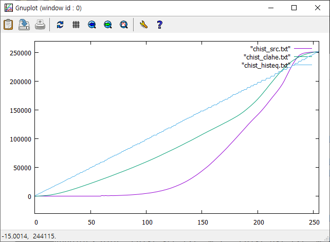
픽셀값의 분포가 좁은 구간에 한정된 영상은 낮은 명암 대비(contrast)를 가지게 된다. 이 경우 픽셀값을 가능한 넓은 구간에 재분포하도록 변환시키면 전체적으로 훨씬 높은 contrast를 가지는 영상을 얻을 수 있는데 이러한 기법을 histogram equalization이라고 한다. Histogram equalization은 픽셀 분포의 cdf(cumulative distribution function)가 가능한 직선이 되도록 변형을 시킨다. 그러나 어떤 경우에는 과도한 contrast로 인해서 영상의 질이 더 안 좋아지는 경우가 발생하거나 영상의 일부 영역에서는 오히려 contrast가 감소하는 경향이 발생할 수 있다. 이를 개선하기 위해는 cdf의 과도한 변형을 막고, equaliztion을 국소적으로 다르게 적용할 수 있는 adaptive 알고리즘을 고려해야 한다. 픽셀값의 분포를 연속적 변수로 생각하면 히스토그램 $h(x)$은 픽셀값의 pdf(probability density function)를 형성하고, 히스토그램의 최댓값과 최솟값을 각각 $m=\text{min}(h)$, $M=\text{max} (h)$라면
$$ m \le \frac{1}{255}\int_0^{255} h(x) dx \le M$$
Histogram equalization은 $m \approx M$이 되도록 $h(x)$을 변환을 시키는 과정에 해당한다. Histogram 함수는 cdf함수의 미분값이므로 cdf 곡선의 접선의 기울기에 해당하고, histogram equation은 cdf 함수의 기울기가 모든 픽셀값에서 일정하게 조정하는 과정이 된다. 과도한 contrast를 갖는 영상을 만들지 않기 위해서 일정한 cdf의 기울기를 요구하지 않고 일정범위를 넘어서는 경우만 제한을 두도록 하자. 제한값은 cdf의 평균변화율
$$\overline{s}=\frac{1}{255}\int_0^{255} h(x) dx$$
을 기준으로 선택하면 된다. 제한 기준으로 $slope \times \overline{s}$를 선택하면 변형된 histogram은
$$ h_\text{modified} (x) = \left\{ \begin{matrix} slope \times \overline{s} & \text{if} ~~h(x) \ge slope \times \overline{s} \\h(x) & \text{otherwise} \end{matrix} \right.$$
확률을 보존하기 위해 기준을 넘는 픽셀 분포는 초과분을 histogram의 모든 bin에 고르게 재분배를 하는 과정이 필요하다.
$$h_\text{modified}(x) \underset{\text{redistribution of excess}}{\Longrightarrow}\tilde{h}_\text{modified}(x)$$
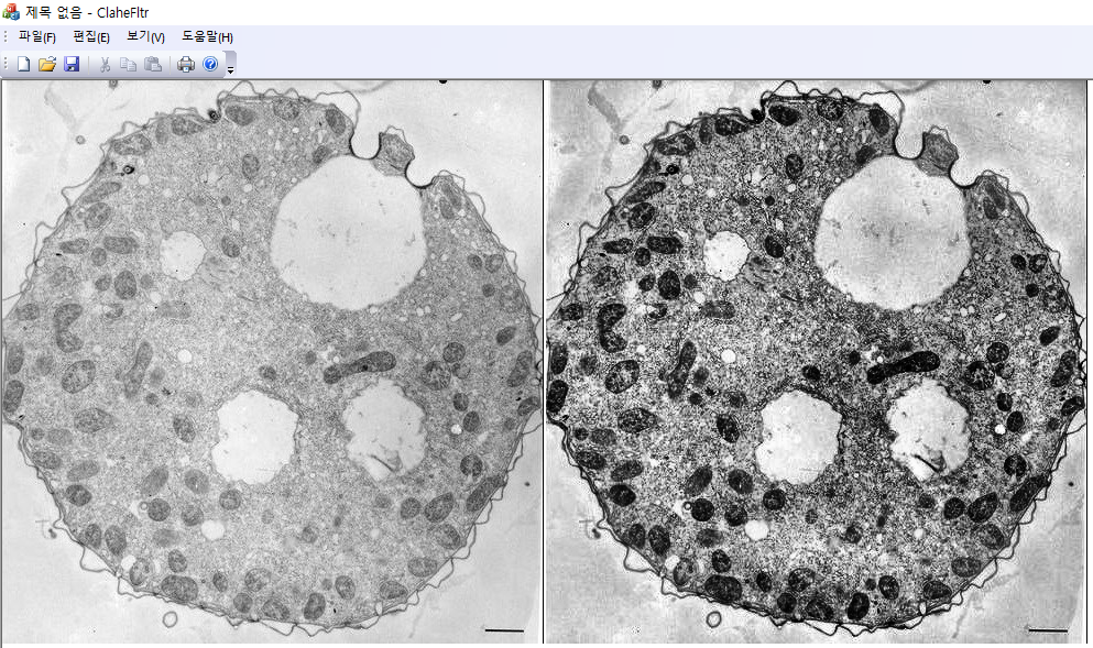
이 새로이 변환된 histogram에 대해 equalization을 적용하여 윈도 중심 픽셀의 값을 설정한다. 이 알고리즘을 contrast limited histogram equalization(CLAHE)라고 부른다. 보통 CLAHE 알고리즘에서는 각각의 픽셀에 대해 윈도를 선택하지 않고, 원본 영상을 겹치는 타일영역으로 분할한 후 각각의 타일에서 제한된 histogram equalization을 변환을 구한다. 그리고 겹치는 인접 타일에서 변환의 선형보간을 이용하면 타일과 타일 사이에서 계단현상을 막을 수 있다. 여기서는 각각의 픽셀에 대해서 슬라이딩 윈도를 설정하는 방법을 사용한다. 윈도 크기는 영상에서 관심 대상을 충분히 커버할 정도의 크기여야 한다. 또한 $slope$은 보통 $3\sim 4$정도를 선택한다. $slope\to 1$인 경우는 원본 영상과 거의 변화가 없고($h(x) \approx \overline{s}$), $slope\gg 1$이면 재분배되는 픽셀이 없으므로 마지막 단계에서 equalization이 global equalization과 동일하게 된다.
static const int halfwindow	= 63;
static const double slope	= 3;
void clahe2(BYTE **input, int width, int height, BYTE **output) {
    const int bins = 255;
    int hist[bins+1], clippedHist[bins+1];
    for (int y = 0; y < height; ++y) {
        int top = max(0, y - halfwindow);
        int bottom = min(height-1, y + halfwindow);
        int h = bottom - top + 1;

        /* 픽셀 access를 줄이기 위해 sliding 윈도우 기법을 사용함;*/
        memset(hist, 0, sizeof(hist));
        int right0 = min(width-1, halfwindow);	// x=0일 때 오른쪽;
        for (int yi = top; yi <= bottom; ++yi)
            for (int xi = 0; xi < right0; ++xi) // x=right는 다음 step에서 더해짐;
                ++hist[input[yi][xi]];

        for (int x = 0; x < width; ++x) {
            int left = max(0, x - halfwindow );
            int right = x + halfwindow;
            int w = min(width-1, right) - left + 1;
            int npixs = h * w;	// =number of pixels inside the sliding window;

            int limit = int(slope * npixs / bins + 0.5);
            // slope >>1 -->hist_eq;
            /* 윈도우가 1픽셀 이동하면 왼쪽 열은 제거; */
            if (left > 0)
                for (int yi = top; yi <= bottom; ++yi)
                    --hist[input[yi][left-1]];

            /* 윈도우가 움직이면 오른쪽 열을 추가함; */
            if (right < width)
                for (int yi = top; yi <= bottom; ++yi)
                    ++hist[input[yi][right]];

            /* clip histogram and redistribute excess; */
            memcpy(clippedHist, hist, sizeof(hist));
            int excess = 0, excessBefore;
            do {
                excessBefore = excess;
                excess = 0;
                for (int i = 0; i <= bins; ++i) {
                    int over = clippedHist[i] - limit;
                    if (over > 0) {
                        excess += over;
                        clippedHist[i] = limit;
                    }
                }

                int avgExcess = excess / (bins + 1);
                int residual  = excess % (bins + 1);// 각 bin에 분배하고 남은 나머지;
                for (int i = 0; i <= bins; ++i)	// 먼저 전구간에 avgExcess를 분배;
                    clippedHist[i] += avgExcess;

                if (residual != 0) {
                    int step = bins / residual;	// 나머지는 일정한 간격마다 1씩 분배;
                    for (int i = 0; i <= bins; i += step)
                        ++clippedHist[i];
                }
            } while (excess != excessBefore);

            /* clipped histogram의 cdf 구성;*/
            int hMin = bins;
            for (int i = 0; i < hMin; ++i)
                if (clippedHist[i] != 0) hMin = i;
            int cdfMin = clippedHist[hMin];

            int v = input[y][x]; //현 위치의 픽셀 값;
            int cdf = 0;
            for (int i = hMin; i <= v; ++i) // cdf(현 픽셀);
                cdf += clippedHist[i];

            int cdfMax = cdf;
            for (int i = v + 1; i <= bins; ++i) // 총 픽셀;
                cdfMax += clippedHist[i];

            // 현픽셀 윈도의 clipped histogram을 구하고,
            // 이 clipped histogram을 써서 equaliztion을 함;
            output[y][x] = int((cdf - cdfMin)/double(cdfMax - cdfMin) * 255);
        }
    }
}Contrast Limited Adaptive Histogram Equalization (CLAHE)
Contrast Limited Adaptive Histogram Equalization (CLAHE). CLAHE는 영상의 평탄화 (histogram equalization) 과정에서 contrast가 과도하게 증폭이 되는 것을 방지하도록 설계된 adaptive algorithm의 일종이다. CLAHE algorithm은
kipl.tistory.com
'Image Recognition > Fundamental' 카테고리의 다른 글
| FFT를 이용한 inverse FFT (0) | 2024.07.31 |
|---|---|
| FFT 구현 (0) | 2024.07.31 |
| Approximate Distance Transform (0) | 2024.06.02 |
| Graph-based Segmentation (1) | 2024.05.26 |
| Linear Least Square Fitting: perpendicular offsets (0) | 2024.03.22 |


