Spline은 일정한 매개변수 구간 $[a, b]$에서 분포된 값(다차원인 경우는 벡터)을 이용해서 만든 다항식을 의미한다. 매개변수 구간 $[a, b]$는 값이 주어진 부분구간들의 합으로 표현할 수 있는데 이 부분구간의 시작과 끝에 해당하는 매개변수 값을 knot이라고 한다. knot이 매개변수 구간 $[a, b]$에 균일하게 퍼져 있는 경우는 uniform spline, 그렇지 않은 경우는 non-uniform spline이라고 한다.

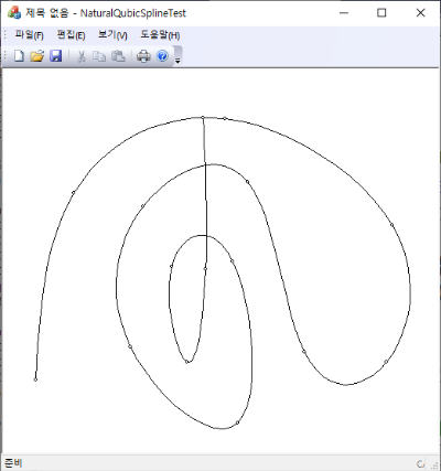
Catmull-Rom spline은 3차 다항식으로 써지는 uniform spline으로 각 knot 위치에서 주어진 값을 통과하므로 interpolation 함수이기도 한다. 그리고 1차 도함수가 연속성을 가지고 있고, knot의 위치 변화나 knot에서 주어진 값의 변화에 곡선이 민감하게 변하지 않는다. 그러나 2차원 이상에는 Catmull-Rom spline이 꼬이는 현상이 발생할 수 있고, 극단적으로는 cusp가 생기는 단점도 가지고 있다.

2차원 이상에서는 Catmull-Rom spline으로 주어진 점(벡터)들을 보간하는 곡선을 찾을 때 uniform이 아니면 knot을 정하는데 모호함이 존재한다. 보통은 순차적으로 주어진 입력점의 직선거리를 이용해서 knot을 정할 수 있는데 이 경우를 chordal Catmull-Rom spline이라고 한다.

주어진 입력점이 $\{{\bf P}_0, {\bf P}_1, {\bf P}_2, {\bf P}_3\}$일 때 knot은

$$ t_i = t_{i-1}+ ||{\bf P}_i – {\bf P}_{i-1}||$$

더 일반적으로 

$$ t_i = t_{i-1} + ||{\bf P}_i - {\bf P}_{i-1}||^\alpha, ~~~\alpha \in [0,1]$$

로 잡을 수 있는데 이 경우를 centripetal Catmull-Rom spline이라 하며 cusp를 피할 수 있다. 단, 입력점의 중복이 없도록 미리 제거되어야 한다. Spline ${\bf S}(t)$는 ${\bf P}_1$과 ${\bf P}_2$사이에서

  • 3차 함수로 쓰여져야 하고,
  • 입력점 통과: ${\bf S}(t_1) = {\bf P}_1$, ${\bf S}(t_2) ={\bf P}_2$ ,
  • 기울기: ${\bf S}'(t_1)=\frac{1}{t_2-t_0} ({\bf P}_2 - {\bf P}_0)$, $ {\bf S}'(t_2) = \frac{1}{t_3-t_1}({\bf P}_3 - {\bf P}_1)$

인 조건을 사용하면 ${\bf S}(t)$에 대한 closed form을 얻을 수 있다(참고: 위키피디아). ${\bf S}(t)$은 $t_1\le t\le t_2$ 사이에서 정의되고, 곡선을 그릴 때 매개변수를 $t\in [0:1]$ 으로 잡으면 ${\bf S}(t)$를 호출할 때는 $t_1 +  (t_2-t_1)t$를 인자로 사용하면 된다.

ref: http://www.cemyuksel.com/research/catmullrom_param/catmullrom.pdf

https://kipl.tistory.com/226


Catmull-Rom Spline

두 개의 점이 주어지는 경우 이들을 잇는 가장 단순한 곡선은 직선이다. 또 직선은 두 점을 잇는 가장 짧은 거리를 갖는 곡선이기도 하다. 그러면 $N$개의 점이 주어지는 경우는 이들 모두 지나는

kipl.tistory.com


red=centripetal Catmull-Rom Spline

double GetParam(double t, double alpha, const CfPt& p0, const CfPt& p1 ) {
    CfPt p = p1 - p0;
    double dsq = p.x * p.x + p.y * p.y;
	if (dsq == 0) return t;
    return pow(a, alpha / 2) + t;
}
//centripetal catmull-rom spline;
CfPt CRSplineA(double t /*[0:1]*/, 
               const CfPt& p0, 
               const CfPt& p1, 
               const CfPt& p2, 
               const CfPt& p3, double alpha=.5 /*[0:1]*/)
{
    double t0 = 0;
    double t1 = GetParam( t0, alpha, p0, p1 );
    double t2 = GetParam( t1, alpha, p1, p2 );
    double t3 = GetParam( t2, alpha, p2, p3 );
    t = t1 * (1 - t) + t2 * t;
    CfPt A1 = t1==t0 ? p0: p0*(t1-t)/(t1-t0) + p1*(t-t0)/(t1-t0);
    CfPt A2 = t2==t1 ? p1: p1*(t2-t)/(t2-t1) + p2*(t-t1)/(t2-t1);
    CfPt A3 = t3==t2 ? p2: p2*(t3-t)/(t3-t2) + p3*(t-t2)/(t3-t2);
    CfPt B1 = A1 * (t2-t)/(t2-t0) + A2 * (t-t0)/(t2-t0);
    CfPt B2 = A2 * (t3-t)/(t3-t1) + A3 * (t-t1)/(t3-t1);
    return B1 * (t2-t)/(t2-t1) + B2 * (t-t1)/(t2-t1);
}
void DrawCatmullRom(std::vector<CfPt>& Q, CDC *pDC) {  
#define STEPS (20)
    if (Q.size() < 4) return ;
    CPen red(PS_SOLID, 2, RGB(255, 0, 0));
    CPen *pOld = pDC->SelectObject(&red);
    const int n = Q.size();
    // centripetal Catmull-Rom spline;
    for (int i = 0; i < n - 1; i++) {
        pDC->MoveTo(Q[i]);
        // i = 0 인 경우에는 처음 점을 반복, i = n - 2인 경우에는 마지막 점을 반복..
        int ip = max(i - 1, 0);
        int inn = min(i + 2, n - 1);
        for (int it = 1; it <= STEPS; it++)
            pDC->LineTo(CRSplineA(double(it)/STEPS, Q[ip], Q[i], Q[i + 1], Q[inn]));
    };
    pDC->SelectObject(pOld);
    CPen blue(PS_SOLID, 2, RGB(0, 0, 255));
    pOld = pDC->SelectObject(&blue);
    // uniform Catmull-Rom spline;
    for (int i = 0; i < n - 1; i++) {
        pDC->MoveTo(Q[i]);
        // i = 0 인 경우에는 처음 점을 반복, i = n - 2인 경우에는 마지막 점을 반복..
        int ip = max(i - 1, 0);
        int inn = min(i + 2, n - 1);
        for (int it = 1; it <= STEPS; it++)
            pDC->LineTo(CRSpline(double(it)/STEPS, Q[ip], Q[i], Q[i + 1], Q[inn]));
    };
    pDC->SelectObject(pOld);
}
728x90

'Computational Geometry' 카테고리의 다른 글

Natural Cubic Spline: revisited  (0) 2024.06.14
Polygon Decimation  (0) 2024.06.08
Bezier curves  (1) 2024.04.19
Subdividing a Bezier Curve  (0) 2024.04.18
Derivatives of Bezier Curves  (1) 2024.04.12
,
 

구간 $[a=t_0, ...t_{n-1}=b]$에서 일정한 간격(꼭 일정한 간격일 필요는 없지만 여기서는 1로 선택함)으로 샘플링된 데이터 $\{ f_0, ...f_{n-1} \}$이 있다. $n-1$ 개의 각 구간에서 데이터를 보간하는 삼차다항식 함수 모임 $$S(t)= \{S_j (t)| t_j \le t <t_{j+1} ,  ~~j=0,1,2...,n-2 \} $$을 찾아보자. 전체 구간에서 연속적이고 충분히 부드럽게 연결되기 위해서는 우선 각 node에서 연속이어야 하고, 또한 1차 도함수와 2차 도함수도 연속이 되어야 한다.  물론 각 node에서는 샘플링된 데이터값을 가져야 한다. 

\begin{align}     (a) ~~& S(t_j) = f_j \\ (b)~~& S_{j+1}(t_{j+1}) = S_j( t_{j+1}) \\ (c)~~& S'_{j+1}(t_{j+1}) = S'_j(t_{j+1}) \\ (d)~~& S''_{j+1}(t_{j+1})  = S''_{j}(t_{j+1}) \end{align}

$n-1$개 구간에서 각각 정의된  3차 함수를 결정하려면 $4 \times (n-1)$개의 조건이 필요하다. (a)에서 $n$개, (b), (c), (d)에서 $3\times (n-2)$개의 조건이 나오므로 총 $n+3\times(n-2)=4n-6$개의 조건만 생긴다. 삼차식을 완전히 결정하기 위해서는 2개의 추가적인 조건을 부여해야 하는데 보통 양끝에서 2차 도함수값을 0으로 하거나(natural boundary) 또는 양끝에서 도함수 값을 특정한 값으로 고정시킨다(clamped boundary). 여기서는 양끝의 2차 도함수를 0으로 한 natural cubic spline만 고려한다. 그리고 $S_j(t)$가 $n-2$개의 구간에 대해서만 정의되어 있지만, 끝점을 포하는 구간에서도 정의하자. 이 경우 $S_{n-1}(t), t\ge t_{n-1}$에 부여된 조건은 $t_{n-1}$에서 $S_{n-2}(t)$와 연속, 미분연속 그리고 2차 도함수가 0인 조건만 부여된다.


$j-$번째 구간의 삼차함수를 

$$S_j(t) = a_j + b_j (t - t_j) + c_j (t-t_j)^2 + d_j (t - t_j)^3$$

로 쓰면 (a)에서 

$$ S_j (t_j) = a_j = f_i,~~ j=0,1,..n-2$$

(b)에서 

$$ a_{j+1} =a_j+  b_j + c_j +d_j,~~j=0,1,...,n-2$$

(c)에서 

$$b_{j+1} = b_j + 2c_j+ 3d_j,~~j=0,1,...,n-2 $$

(d)에서 

$$ c_{j+1} = c_j+ 3d_j,~~j=0,1,...,n-2$$

이므로 (b)와 (c)에서 $d_j$을 소거하면

$$  c_j = 3(a_{j+1}-a_j) -b_{j+1} - 2b_j$$

그리고 (a)에서 $$d_j = -2(a_{j+1}-a_j) + b_j  + b_{j+1}$$ 이므로 $b_j$에 대해 정리하면 다음과 같은 점화식을 얻을 수 있다.

$$ b_{j+1} + 4b_j + b_{j-1}= 3(a_{j+1}- a_{j-1})=3(f_{j+1}-f_{j}),~~j=1,2,...,n-2$$

물론 $j=0$일 때는 (note, $S''_0(t_0) = 0 \to c_0=0$) $a_1 =a_0+b_0+d_0, b_1 = b_0 + 3d_0$이므로

$$ b_1 + 2b_0 = 3(f_1 - f_0) $$

$j=n-1$일 때 계수는 $S_{n-1}(t_{n-1}) = f_{n-1}$이고 $S''_{n-1}(t_{n-1} )=c_{n-1}=0$이므로 $$ 2b_{n-1} + b_{n-2} = 3(f_{n-1}-f_{n-2})$$

임을 알 수 있다. 따라서 계수를 구하는 과정은 $b_j~(j=0,...,n-1)$을 구하는 것으로 결정된다. 이를 행렬로 표현하면

$$ \begin{bmatrix} 2&1& \\1&4&1\\ &1&4&1 \\ & & & \cdots \\ &&&&1&4&1  \\ && & & & 1 &2 \end{bmatrix} \begin{bmatrix} b_0\\b_1\\ \vdots \\   b_{n-2} \\b_{n-1}\end{bmatrix}=\begin{bmatrix} 3(f_1-f_0) \\ 3(f_2-f_0) \\  \vdots \\  3(f_{n-1}- f_{n-3}) \\3(f_{n-1} - f_{n-2}) \end{bmatrix}$$

와 같다. band 행렬은 upper triangle로 변환한 후 역치환과정을 거치면 쉽게 해를 구할 수 있다.


평면에서 주어진 점들을 보간하는 곡선은 이들 점을 표현하는 곡선의 매개변수를 일정한 간격으로 나누어서 샘플링된 결과로 취급하면, $x, y$ 성분에 대해서 각각 natural cubic spline를 구하여 얻을 수 있다. 그러나 곡선이 급격히 변할 때는 매개변수를 일정하게 잡는 것보다는 입력점의 사이거리를 기준으로 선택하는 것이 더 유연한 보간곡선을 만들어 준다.

struct Cubic {
    double a,b,c,d;  /* a + b*t + c*t^2 +d*t^3 */
    Cubic() {}
    Cubic(double a_, double b_, double c_, double d_) 
        : a(a_), b(b_), c(c_), d(d_) { }
    /* evaluate;*/
    double eval(double t) {
        return (((d*t) + c)*t + b)*t + a;
    }
};
std::vector<Cubic> calcNaturalCubic(std::vector<double>& x) {
    std::vector<double> gamma(x.size());
    std::vector<double> delta(x.size());
    std::vector<double> D(x.size());
    /* solve the banded equation:
    [2 1       ] [  D[0]]   [3(x[1]   - x[0])  ]
    |1 4 1     | |  D[1]|   |3(x[2]   - x[0])  |
    |  1 4 1   | | .    | = |      .           |
    |    ..... | | .    |   |      .           |
    |     1 4 1| | .    |   |3(x[N-1] - x[N-3])|
    [       1 2] [D[N-1]]   [3(x[N-1] - x[N-2])]
    ** make the banded matrix to an upper triangle;
    ** and then back sustitution. D[i] are the derivatives at the nodes.
    */
    const int n = x.size() - 1;  // note n != x.size()=N;
    // gamma;
    gamma[0] = 0.5;
    for (int i = 1; i < n; i++)
        gamma[i] = 1/(4-gamma[i-1]);
    gamma[n] = 1/(2-gamma[n-1]);
    // delta;
    delta[0] = 3*(x[1]-x[0])*gamma[0];
    for (int i = 1; i < n; i++) 
        delta[i] = (3*(x[i+1]-x[i-1])-delta[i-1])*gamma[i];
    delta[n] = (3*(x[n]-x[n-1])-delta[n-1])*gamma[n];
    // D;
    D[n] = delta[n];
    for (int i = n; i-->0;)
        D[i] = delta[i] - gamma[i]*D[i+1];

    /* compute the coefficients;*/
    std::vector<Cubic> Spline(n);
    for (int i = 0; i < n; i++)
        Spline[i] = Cubic(x[i], D[i], 3*(x[i+1]-x[i])-2*D[i]-D[i+1],
                                      2*(x[i]-x[i+1]) + D[i] + D[i+1])) ;
    return Spline;
}
std::vector<CPoint> NaturalCubicSpline(const std::vector<CPoint>& points) {
    if (points.size() < 2) return std::vector<CPoint> (); // null vector;
    std::vector<double> xp(points.size()), yp(points.size());
    for (int i = points.size(); i-->0;)
        xp[i] = points[i].x, yp[i] = points[i].y;
        
    std::vector<Cubic> splineX = calcNaturalCubic(xp);
    std::vector<Cubic> splineY = calcNaturalCubic(yp);
#define STEPS 12
    std::vector<CPoint> curve;
    curve.reserve(splineX.size() * STEPS + 1);
    curve.push_back(points.front());
    for (int i = 0; i < splineX.size(); i++) {
        for (int j = 1; j <= STEPS; j++) {
            double t = double(j) / STEPS;
            curve.push_back(CPoint(int(splineX[i].eval(t)+0.5), int(splineY[i].eval(t)+0.5)));
        }
    }
    return curve;
}
728x90

'Computational Geometry' 카테고리의 다른 글

Least Squares Bezier Fit  (0) 2024.04.05
Why Cubic Splines?  (9) 2024.03.16
Approximate Distance Between Ellipse and Point  (0) 2024.03.08
Distance from a Point to an Ellipse  (0) 2024.03.06
Data Fitting with B-Spline Curves  (0) 2021.04.30
,

Lanczos kernel:  a sinc function windowed by the central lobe of a second, longer, sinc function(wikipedia)

$$K(x) = \left\{ \begin {array}{ll}   \text {sinc}(\pi x) \text {sinc}\Big( \frac {\pi x}{a}\Big), & |x| < a \\ 0 ,& |x| \ge a\end {array} \right. = \text{sinc}(\pi x) \text{sinc}\Big( \frac{\pi x}{a}\Big)\text{Box}(|x|<a) $$

$$H(\omega)=\frac{1}{2\pi^2\sqrt{2\pi}}\Big( -(2\pi-3\omega)\text{Si}(2\pi-3\omega)+(4\pi -3\omega)\text{Si}(4\pi-3\omega)$$$$+(2\pi +3\omega)\text{Si}(2\pi+3\omega)+(4\pi+3\omega)\text{Si}(4\pi+3\omega)\Big).$$

여기서 sine intergral은 다음과 같이 정의된다:

$$\text{Si}(x)=\int_0^x \frac{\sin(t)}{t} dt.$$

$x=0$ 근방에서는 Tayor 전개식을 이용하는 것이 더 효율적인다.

\

Lanczos kernel을 사용해서 일정한 간격으로 sampling 된 데이터 $\{f_i \}$를 보간하려고 할 때 보간함수 $F(x)$는 Lanczos kernel과 데이터의 convolution으로 표현할 수 있다.

$$ F(x) = \sum_{i \in \text{window}} f_i K(x - i) $$

Interpolation 함수는 영상의 resampling 과정에서 사용할 수 있다. 주어진 이미지를 확대하거나 축소하려면 기존 이미지의 픽셀과 픽셀 사이 구간에서 픽셀 값을 알아내야 하는데, 이때 interpolation 함수를 이용하여 필요한 데이터를 얻는 과정인 resampling 한다.


다음 코드는 Lanczos3 kernel을 사용해서 이미지를 확대하거나 축소할 때 행에 대해서 필요한 resampling을 수행한다. 여기서는 kernel의 중심이 소스 이미지의 픽셀과 픽셀의 가운데에 놓이도록 설정하였다($-0.5$의 의미). 이는 작은 영상을 크게 확대할 때 가장자리에서 왜곡이 되는 것을 방지하기 위해서 인데 큰 영상을 확대/축소할 때는 영향이 없다. 이 interpolation은 separable이므로 2차원의 경우 행방향으로 진행한 후 그 결과를 다시 열 방향으로 진행하는 2-pass 방식으로 사용해도  된다.

// windowed sinc(x); window=sinc(x/3);
static double Lanczos3(double x){
    if (x < 0) x = -x; // symmetric;
    x *= PI;
    if (x < 0.01)    return 1. + (- 5./ 27. + 
        (14. / 1215. - 17. * x * x / 45927.) * x * x) * x * x; 
    else if (x < 3.) return 3. * sin(x) * sin(x / 3.) / x / x;
    else     	     return 0;
};
// interpolation in the horizonal direction: single channel or gray image;
// x = pixel position in a destination image;
double Lanczos3_line(BYTE *src_line, int srcWidth, int x, double xscale) {
    double halfWidth;
    if (xscale > 1.) halfWidth = 3.;
    else             halfWidth = 3. / xscale;

    double centerx = double(x) / xscale - 0.5;  //center loc of filter in the src_line;
    int left  = (int)floor(centerx - halfWidth);
    int right = (int)ceil(centerx + halfWidth);
    if (xscale > 1) xscale = 1;
    double s = 0;
    double weightSum = 0;
    for (int ix = left; ix <= right; ix++) {   
        double weight = Lanczos3((centerx - ix) * xscale);
        // for ix<0 || ix>=srcWidth: repeat boundary pixels
        int xx = min(max(ix, 0), srcWidth - 1));
        s += weight * src_line[xx];
        weightSum += weight;
    }
    return s / weightSum; 
}


이차원 이미지의 경우 수평방향의  적용한 후 다시 수직방향으로 적용하면 된다. 

bicubic downsample(1/2): alias 발생

// 수평-수직을 동시함; 2 pass version으로 바꾸는 것이 더 효율적임;
void Lanczos3ResampleRGB(BYTE *src, int srcWidth, int srcHeight, 
                         BYTE *dst, int dstWidth, int dstHeight)
{
    const int bytes = 3; // = 1 for gray;
    const double xscale = double(dstWidth) / srcWidth;
    const double yscale = double(dstHeight) / srcHeight;
    double halfWidth, scale;
    if (yscale > 1.) {
        halfWidth = 3; scale = 1;
    }
    else {
        halfWidth = 3 / yscale; scale = yscale;
    }
    double color[3];
    for (int y = 0; y < dstHeight; ++y) {
        BYTE *pdst = &dst[y * dstWidth * bytes];
        for (int x = 0; x < dstWidth; ++x) {
            double csum[3] = {0}, weightSum = 0;
            // dst geometry;
            double centery = double(y) / yscale - 0.5;
            int top = (int)floor(centery - halfWidth);
            int bot = (int)ceil(centery + halfWidth);
            for (int iy = top; iy <= bot; ++iy) {
                double weight = Lanczos3((centery - iy) * scale);
                int ys = max(0, min(iy, srcHeight - 1));
                weightSum += weight;
                Lanczos3_lineRGB(&src[ys * srcWidth * bytes], srcWidth, x, xscale, color);
                for (int c = 0; c < bytes; ++c) 
                    csum[c] += weight * color[c];
            }
            for (int c = 0; c < bytes; ++c) {
                int a = int(csum[c] / weightSum);
                *pdst++ = a < 0 ? 0: a > 255 ? 255: a;
            }
        }
    }
}
728x90

'Image Recognition > Fundamental' 카테고리의 다른 글

Poisson Image Editing  (0) 2021.08.03
Sampling Theorem  (0) 2021.05.12
Interpolation Kernels  (0) 2021.05.05
Fowler Angle  (0) 2021.04.05
Brute-Force Euclidean Distance Transform  (0) 2021.03.14
,