Geometry & Recognition

주어진 데이터를 잘 피팅하는 직선을 찾기 위해서는 데이터를 이루는 각 점의 $y$ 값과 같은 위치에서 구하려는 직선과의 차이 (residual)의 제곱을 최소화시키는 조건을 사용한다. 그러나 직선의 기울기가 매우 커지는 경우에는  데이터에 들어있는 outlier에 대해서는 그 차이가 매우 커지는 경우가 발생할 수도 있어 올바른 피팅을 방해할 수 있다. 이를 수정하는 간단한 방법 중 하나는 $y$값의 차이를 이용하지 않고 데이터와 직선 간의 최단거리를 이용하는 것이다. 

수평에서 기울어진 각도가 $\theta$이고 원점에서 거리가 $s$인 직선의 방정식은 

$$ x \sin \theta - y \cos \theta + s=0$$

이고, 한 점 $(x_i, y_i)$에서 이 직선까지 거리는

$$ d_i = | \sin \theta y_i - \cos \theta x_i + s|$$

이다. 따라서 주어진 데이터에서 떨어진 거리 제곱의 합이 최소인 직선을 구하기 위해서는 다음을 최소화시키는 $\theta, s$을 구해야 한다. $$ L = \sum_i \big( \sin \theta x_i - \cos \theta y_i +s \big)^2 \\ (\theta, s)=\text{argmin}(L)$$

$\theta$와 $s$에 대한 극값 조건에서 

$$\frac{1}{2} \frac{\partial L}{\partial \theta} = \frac{1}{2} \sin 2 \theta \sum_i (x_i^2 - y_i^2) - \cos 2 \theta \sum x_i y_i + s \sin \theta \sum_i x_i + s \cos \theta \sum_i y_i = 0$$

$$ \frac{1}{2}\frac{\partial L}{\partial s}=\cos \theta \sum y_i  - \sin \theta \sum_i x_i - N s=0$$

주어진 데이터의 질량중심계에서 계산을 수행하면 $\sum_i x_i = \sum_i y_i =0$ 이므로 데이터의 2차 모멘트를 $$ A= \sum_i (x_i^2 - y_i^2), \qquad B = \sum_i x_i y_i $$로 놓으면 직선의 파라미터를 결정하는 식은

$$ \frac{1}{2} A \sin 2 \theta   - B \cos 2 \theta = 0  \qquad \to \quad  \tan 2\theta = \frac{2B}{A} \\ s = 0$$

두 번째 식은 직선이 질량중심(질량중심계에서 원점)을 통과함을 의미한다. 첫번째 식을 풀면

$$ \tan \theta = \frac{- A \pm \sqrt{A^2 + (2B)^2 }}{2B}$$

두 해 중에서 극소값 조건을 만족시키는 해가 직선을 결정한다. 그런데

$$ \frac{1}{2}\frac{\partial^2 L}{\partial \theta^2}=  A \cos 2 \theta + 2B \sin 2 \theta = \pm \sqrt{A^2 + (2B)^2}  >0$$

이므로 위쪽 부호로 직선($x\sin \theta = y\cos \theta$)이 정해진다. 질량중심계에서는 원점을 지나지만 원좌표계로 돌아오면 데이터의 질량중심을 통과하도록 평행이동시키면 된다.

$$  \left(-A+ \sqrt{A^2+ (2B)^2} \right)  (x-\bar{x}) = 2B (y - \bar{y})  $$

여기서 주어진 데이터의 질량중심은 원좌표계에서

$$ \bar{x} = \frac{1}{N} \sum_i x_i, \quad \bar{y} = \frac{1}{N} \sum_i y_i$$

이다. 또한 원좌표계에서 $A$와 $B$의 계산은 

$$ A = \sum_i [ (x_i - \bar{x})^2 - (y_i - \bar{y})^2], \qquad B = \sum (x_i  - \bar{x})(y_i - \bar{y})$$ 

이 결과는 데이터 분포에 PCA를 적용해서 얻은 결과와 동일하다. PCA에서는 공분산 행렬의 고유값이 큰 쪽에 해당하는 고유벡터가 직선의 방향을 결정했다. https://kipl.tistory.com/211.  또한 통계에서는 Deming regression이라고 불린다.

일정한 간격 $h$마다 샘플링된 데이터 $\{ (x_k, f_k) \}$를 이용해서 이들 데이터를 표현하는 spline를 구해보자. spline은 주어진 샘플링 데이터을 통과할 필요는 없으므로 일반적으로 interpolation 함수는 아니다. 이 spline은 샘플링 데이터와 kernel이라고 불리는 함수의 convolution 형태로 표현할 수 있다.

$$ g(x) = \sum_k  f_k K \left( \frac{x-x_k}{h}\right)$$

이미지의 resampling 과정에서 spline를 이용하는데 이때 사용 가능한 kernel의 형태와 그 효과를 간단히 알아보자.

3차 spline kernel은 중심을 기준으로 반지름이 2인 영역 $(-2,1),(-1,0), (0,1), (1,2)$에서만  0이 아닌 piecewise 삼차함수다. 그리고 이 함수는 우함수의 특성을 갖는다. 따라서 가능한 형태는

$$ K(s) = \left\{ \begin{matrix} A_1|s|^3 + B_1 |s|^2 +C_1 |s| + D_1    &  |s| <1 \\ A_2 |s|^3 + B_2 |s|^2 + C_2 |s| + D_2 & 1 \le |s|<2 \\ 0 & \text{otherwise} \end{matrix} \right. $$처럼 쓸 수 있다. 계수를 완전히 결정하기 위해서는 8개의 조건이 필요한다. 우선 우함수이므로 원점에서 미분값이 제대로 정의되려면 $$C_1=0$$도 만족해야 한다, 그리고 각 node에서 연속성을 요구하면

\begin{align} s=1^\pm:~~~& A_1+B_1 +D_1 = A_2 +B_2+C_2 +D_2 \\ s=2^\pm:~~~& 8A_2 +4B_2 +2C_2 +D_2 =0 \end{align} 임을 알 수 있다. 또한 각 node에서 부드럽게 연결되기 위해서 1차 도함수가 연속적임을 요구하면

\begin{align} s = 1^\pm:~~~& 3A_1 + 2B_1 = 3A_2 + 2B_2+C_2 \end{align}

그리고 샘플링된 데이터가 모두 같은 경우 보간함수도 상수함수가 되는 것이 타당하므로

$$ g(x) = \sum_k K \left( \frac{x-x_k}{h}\right) = 1~~~\text{if} ~~\forall f_j = 1$$

을 만족시켜야 한다. $x_j <x<x_{j+1}$일 때 $x  =  x_j + sh,  ~(0< s<1)$로 쓸 수 있고, kernel이 반지름이 2인  support를 가지므로 

$$ g(x) =  K(s+1) + K(s) +  K(s-1) + K(s-2)=1$$

임을 알 수 있다. 위에서 주어진 $K(s)$을 대입해서 정리하면 다음과 같은 항등식을 얻는다.

$$ -1 + A_1 + 9 A_2 + B_1 + 5 B_2 + 3 C_2 + 2 D_1 +2 D_2 \\ +(-3 A_1 - 9 A_2 - 2 B_1 - 2 B_2) s + (3 A_1 + 9 A_2 + 2 B_1 + 2 B_2) s^2 =0$$

이 항등식의 계수가 0이 되어야 한다는 사실에서 2 개의 추가 조건을 얻으므로 총 8개 계수 중 2개가 미결정 free parameter로 남는다. 보통 이 두 계수는 $D_1=1-B/3$,  $D_2=4C + 4B/3$처럼 매개화한다. 이 경우 kernel 함수는

$$ K(s)  = \frac{1}{6} \left\{ \begin{matrix}   (12-9B-6C)|s|^3 +(-18+12B+6C) |s|^2 + (6-2B) & |s|< 1\\ (-B-6C)|s|^3 +(6B+30C)|s|^2 + (-12B-48C) |s| + (8B+24C) & 1\le |s|<2\\0 & \text{otherwise} \end{matrix} \right.$$

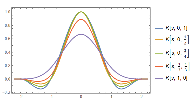
따라서 cubic spline kernel은 두 개의 파라미터 (B,C)에 의해서 정해진다. 또한 kernel 함수의 적분은 $B,C$에 상관없이 항상 1이어서 총 가중치의 합이 1임이 자동으로 보증된다.

$$\int_{-\infty}^\infty K(s)ds =1$$

이 중에는 이미지의 resampling에서 많이 사용되는 커널도 있는데, 잘 알려진 경우를 보면

$$ \begin{matrix} (B,C)=(0,1) & \text{Cardinal spline} \\ (B,C)=(0,1/2) & \text{Catmull-Rom spline } \\ (B,C)=(0,3/4) & \text{used in photoshop} \\ (B,C)=(1/3,1/3) & \text{ Mitchell-Netravali spline}  \\ (B,C)=(1,0) & \text{B-spline}\end{matrix}$$

$B=0$인 경우는 $s=0$일 때 1이고, $|s|=1,2$일 0이므로 interpolation kernel($K(i-j)=\delta_{ij}$)에 해당한다. 그리고 $B=0, C=1/2$인 경우인 Catmul-Rom spline은 node에서 2차 도함수까지도 연속이므로 샘플링 데이터를 생성한 원 아날로그 함수에 $O(h^3)$이내에서 가장 유사하게 근사함을 보일 수도 있다.

// Mitchell Netravali Reconstruction Filter
// B = 0    C = 0   - Hermite B-Spline interpolator 
// B = 0,   C = 1/2 - Catmull-Rom spline
// B = 1/3, C = 1/3 - Mitchell Netravali spline
// B = 1,   C = 0   - cubic B-spline
double MitchellNetravali(double x, double B, double C) {
    x = fabs(x);
    if (x >= 2) return 0;
    double xx = x*x;
    if (x >= 1) return ((-B - 6*C)*xx*x 
                + (6*B + 30*C)*xx + (-12*B - 48*C)*x 
                + (8*B + 24*C))/6;
    if (x < 1) return ((12 - 9*B - 6*C)*xx*x +
        (-18 + 12*B + 6*C) * xx + (6 - 2*B))/6;
}

일반적인 conic section 피팅은 주어진 데이터 $\{ (x_i, y_i)\}$를 가장 잘 기술하는 이차식

$$F(x, y) = ax^2 + bxy +cy^2 + dx +ey +f=0 $$

의 계수 ${\bf u^T}= (a,b,c,d,e,f)$을 찾는 문제이다. 이 conic section이 타원이기 위해서는 2차항의 계수 사이에 다음과 같은 조건을 만족해야 한다.

$$\text{ellipse constraint:}~~ ac - b^2/4 >0$$

그리고 얼마나 잘 피팅되었난가에 척도가 필요한데 여기서는 주어진 데이터의 대수적 거리 $F(x,y)$을 이용하자. 주어진 점이 타원 위의 점이면 이 값은 정확히 0이 된다. 물론 주어진 점에서 타원까지의 거리를 사용할 수도 있으나 이는 훨씬 복잡한 문제가 된다.  따라서 해결해야 하는 문제는

\begin{gather}L = \sum _{i}  \left( ax_i^2 + bx_i y_i + cy_i^2 +dx_i + e y_i +f\right)^2 - \lambda( 4ac-b^2-1) \\= \left|\begin{pmatrix}x_0^2& x_0y_0 & y_0^2 & x_0 & y_0 & 1\\ x_1^2 & x_1 y_1& y_1^2 & x_1 & y_1 & 1 \\ x_2^2 & x_2y_2& y_2^2 & x_2& y_2 & 1\\ &&\vdots \\\end{pmatrix}\begin{pmatrix}a\\b\\c\\d\\e\\f \end{pmatrix}  \right|^2 -\lambda \left({\bf  u^T} \begin{pmatrix} 0& 0& 2&0&0&0\\ 0 &-1&0 &0 &0 &0\\ 2&0&0&0&0&0\\0&0&0&0&0&0 \\0&0&0&0&0&0\\0&0&0&0&0&0&  \end{pmatrix} \bf u -1\right) \\ =\bf u^T D^TD u -\lambda (u^T C u -1)\\ = \bf u^T S u -\lambda (u^T C u-1)\end{gather}

을 최소화시키는 계수 벡터 $\bf u$를 찾는 것이다. 여기서 제한조건으로 $4ac - b^2 =1= \bf u^T C u$로 설정했다. 

$\bf u^T$에 대해서 미분을 하면 

$$ \frac{\partial L}{\partial \bf u^T} =  \bf S u -\lambda C u=0$$

즉, 주어진 제한조건 $4ac - b^2=1$하에서 대수적 거리를 최소화시키는 타원방정식의 계수 $\bf u$를 구하는 문제는 scattering matrix $\bf S=D^T D$에 대한 일반화된 고유값 문제로 환원이 된다.

$$  \bf S u =\lambda C u \\ u^T C u =1$$

이 문제의 풀이는 직전의 포스팅에서 다른 바 있는데 $\bf S$의 제곱근 행렬 $\bf Q=S^{1/2}$를 이용하면 된다. 주어진 고유값 $\lambda$와 고유벡터 $\bf u$가 구해지면 대수적 거리는 $$\bf u^T S u = \lambda$$

이므로 이를 최소화시키기 위해서는 양의 값을 갖는 고유값 중에 최소에 해당하는 고유벡터를 고르면 된다. 그런데 고유값 $\lambda$의 부호별 개수는 $\bf C$의 고유값 부호별 개수와 동일함을 보일 수 있는데 (Sylverster's law of inertia),  $\bf C$의 고유값이 $\{-2,-1,2,0,0,0\}$이므로 $\lambda>0$인 고유값은 1개 뿐임을 알 수 있다. 따라서 $\bf S u = \lambda C u$를 풀어서 얻은  유일한 양의 고유값에 해당하는 고유벡터가 원하는 답이 된다.

https://kipl.tistory.com/370

https://kipl.tistory.com/565

 Ref: https://www.microsoft.com/en-us/research/wp-content/uploads/2016/02/ellipse-pami.pdf

double FitEllipse(std::vector<CPoint>& points, double einfo[6] ) {     
    if ( points.size() < 6 ) return -1;
    double eigvals[6];
    std::vector<double> D(6 * points.size());
    double S[36];/*  S = ~D * D  */
    double C[36];
    double EIGV[36];/* R^T; transposed orthogonal matrix;*/

    double offx = 0, offy = 0;
    /* shift all points to zero */
    for(int i = points.size(); i--> 0; ) {	
        offx += points[i].x;
        offy += points[i].y;        	
    }
    offx /= points.size(); 
    offy /= points.size();

    /* for the sake of numerical stability, scale down to [-1:1];*/
    double scale = 0; 
    for (int i = points.size(); i-->0; ) {
        if (points[i].x > scale) scale = points[i].x;
        if (points[i].y > scale) scale = points[i].y;
    }
    double invscale = 1 / scale;
    /* ax^2 + bxy + cy^2 + dx + ey + f = 0*/
    /* fill D matrix rows as (x*x, x*y, y*y, x, y, 1 ) */
    for(int i = points.size(); i--> 0; ) {	
        double x = points[i].x - offx; x *= invscale; 
        double y = points[i].y - offy; y *= invscale;
        D[i*6 + 0] = x*x; D[i*6 + 1] = x*y;
        D[i*6 + 2] = y*y; D[i*6 + 3] = x;
        D[i*6 + 4] = y;   D[i*6 + 5] = 1;		
    }			

    /* scattering matrix: S = ~D * D (6x6)*/
    for (int i = 0; i < 6; i++) 
        for (int j = i; j < 6; j++) { /*upper triangle;*/
            double s = 0;
            for (int k = points.size(); k-- > 0; ) 
                s += D[k*6 + i] * D[k*6 + j];
            S[i*6 + j] = s;
        }
    for (int i = 1; i < 6; i++) /*lower triangle;*/
        for (int j = 0; j < i; j++) 	
            S[i*6 + j] = S[j*6 + i] ;
    
    /* fill constraint matrix C */
    for (int i = 0; i < 36 ; i++ ) C[i] = 0;
    C[12] =  2 ;//2x0 
    C[2 ] =  2 ;//0x2 
    C[7 ] = -1 ;//1x1

    /* find eigenvalues/vectors of scattering matrix; */
    double RT[36];	/* each row contains eigenvector; */
    JacobiEigens ( S, RT, eigvals, 6, 0 );
    /* create R and INVQ;*/
    double R[36];
    for (int i = 0; i < 6 ; i++) {
        eigvals[i] = sqrt(eigvals[i]);
        for ( int k = 0; k < 6; k++ ) {
            R[k*6 + i] = RT[i*6 + k];  /* R = orthogonal mat = transpose(RT);*/
            RT[i*6 + k] /= eigvals[i]; /* RT /= sqrt(eigenvalue) row-wise)*/
        }
    }
    /* create INVQ=R*(1/sqrt(eigenval))*RT;*/
    double INVQ[36];
    _MatrixMul(R, RT, 6, INVQ);

    /* create matrix INVQ*C*INVQ */
    double TMP1[36], TMP2[36];
    _MatrixMul(INVQ, C, 6, TMP1 );
    _MatrixMul(TMP1, INVQ, 6, TMP2 );
    
    /* find eigenvalues and vectors of INVQ*C*INVQ:*/
    JacobiEigens ( TMP2, EIGV, eigvals, 6, 0 );
    /* eigvals stores eigenvalues in descending order of abs(eigvals);*/
    /* search for a unique positive eigenvalue;*/
    int index = -1, count = 0;
    for (int i = 0 ; i < 3; i++ ) {
        if (eigvals[i] > 0) {
            index = i; // break;
            count++;
        }
    }
    /* only 3 eigenvalues must be non-zero 
    ** and only one of them must be positive;*/
    if ((count != 1) || (index == -1)) 
        return -1;
     
    /* eigenvector what we want: u = INVQ * v */
    double u[6]; 
    double *vec = &EIGV[index*6];
    for (int i = 0; i < 6 ; i++) {
        double s = 0;
        for (int k = 0; k < 6; k++) s += INVQ[i*6 + k] * vec[k];
        u[i] = s;
    }
    /* extract shape infos;*/
    PoseEllipse(u, einfo);
    /* recover original scale; center(0,1) and radii(2,3)*/
    for (int i = 0; i < 4; i++) einfo[i] *= scale;
    /* recover center */
    einfo[0] += offx; 
    einfo[1] += offy;
    return FitError(points, offx, offy, scale, u);
};

열방정식에서 매질에서 열의 확산은 특별히 선호된 방향이 없이 모든 방향에 대해서 동등하다. 물론 매질의 열전도도가 다르면 국속적으로 열확산이 균일하지 않을 수는 있어도 방향을 따지는 않는다. 그러면 방향에 따라 열의 확산을 정도를 다르게 설정하려면 어떻게 해야 할까? 이는 열방정식을 이용해서 이미지의 smoothing을 하는 필터에서도 동일한 상황이 생길 수 있다. 특히 에지를 보존하면서 smoothing을 할 때 에지에 수직방향으로는 확산이 잘 안일어나게 억제해야 할 필요가 있다. 이를 위해 2차원 열방정식의 우변을 살펴보자. 우변은 온도 $u(x,y;t)$의 Laplacian이 들어오는데 보다 일반적인 Hessian matrix $H$을 써서 표현하면 그 의미가 더 명확해진다.

$$ H = \begin{pmatrix} u_{xx} & u_{xy}\\ u_{xy} & u_{yy} \end{pmatrix}$$

$$ u_{xx} + u_{yy} = (1, 0).H. \begin{pmatrix} 1 \\0\end{pmatrix}+ (0,1) . H. \left( \begin{matrix} 0 \\1 \end{matrix} \right) = \text{Tr}\left ((e_1 \otimes  e_1^T + e_2 e \otimes _2^T).H\right)$$

즉, Laplacian은 평면에서 두 단위 벡터  $e_1=(1,0)^T$과 $e_2 =(0,1)^T$ 각각에 Hessian을 작용한 결과를 다시 자신과 내적을 한 값을 동일하게 더하여 나온다. 따라서 $x$방향이나 $y$방향에 무관하게 등방적으로 작용하게 된다. 그러나 $x$방향과 $y$방향에 다른 가중치 $\alpha, \beta\ne \alpha$를 둔다면 등방성은 사라지게 될 것이고 가중치가 큰 방향으로 열의 확산이 더 잘 일어나게 된다.

$$ \alpha u_{xx} + \beta u_{yy}= \alpha \times (1, 0).H. \left(\begin{matrix} 1 \\0\end{matrix} \right)+ \beta(0,1) . H. \left( \begin{matrix} 0 \\1 \end{matrix} \right) = \text{Tr}\left((\alpha e_1 \otimes e_1^T + \beta e_2 \otimes e_2^T).H \right)$$  

일반적으로 $x,y$ 방향의 단위벡터 대신에 서로 직각이 단위벡터를 사용해서 비등방성을 줄 수 있다. 예를 들면 에지 방향에 수직한 방향으로 확산을 억제하고 싶은 경우에는 그래디언트의 공변행렬 $\left(\begin{matrix} u_x^2 & u_x u_y\\ u_x u_y& u_y^2 \end{matrix}\right)$의 두 고유벡터 $v_1$, $v_2$를 이용할 수 있다. 이 경우 고유값이 큰 쪽에 해당하는 고유벡터의 방향이 에지에 수직방향이고, 작은 쪽이 에지 방향을 가리킨다. 

$$    \text{Tr}\left( (c_1 v_1 \otimes v_1^T + c_2 v_2 \otimes v_2^T ).H\right) = \text{Tr}(T.H) \\T= c_1 v_1 \otimes v_1^T + c_2 v_2 \otimes v_2^T $$

이 경우 비등방적 확산은 텐서필드 $T$에 의해서 제어가 되고 열(확산)방정식은 다음과 같이 간단한 형식으로 표현할 수 있다.

$$ u_t = \text{Tr} (T.H)$$

텐서필드는 고유벡터의 텐서곱을 선형결합해서 만드는데 계수 $c_1$과 $c_2$를 어떻게 선택하는가에 따라 확산의 유형이 달라진다. 에지를 보존하도록 컨트롤하기 위해서는 고유값이 큰 방향으로 가중치가 작게 되도록 선택을 해야 한다. 많이 사용되는 예로는 고유값이 각각 $\lambda_1 < \lambda_2$일 때

$$ c_ 1 = (1 + (\lambda_1 + \lambda_2)/s)^{-p_1},  ~~c_2 = (1+ (\lambda_1 + \lambda_2)/s)^{-p_2}, ~~0<p_1 < p_2$$ 

로 잡는다.

void AnisoDiffusion(double **image, int width, int height) {
    // preparation;
    // ....

    // main iteration loop
    for (int iter = 0; iter < max_iter; iter++) {
        // compute gradients;
        Gradient(image, width, height, Gx, Gy);
        // compute the tensor field T, used to drive the diffusion
        for (int x = width; x-- > 0;) {
            for (int y = height; y-- > 0;) {			
                // covariance matrix;
                double a = Gx[x][y] * Gx[x][y]; 
                double b = Gx[x][y] * Gy[x][y];
                double d = Gy[x][y] * Gy[x][y];
                // eigenvalues of symm matrix [a,b;b,d]
                double lambda1, lambda2;
                Eigenvalues(a, b, d, lambda1, lambda2); // 0 <= lambda1 <= lambda2;
                // eigenvector for lambda1; ev1=(u,v);
                double u, v;
                Eigenvector(a, b, d, lambda1, u, v);
                // eigenvector for lambda2: ev2=(-v,u);

                double val1 = lambda1 / drange2; 
                double val2 = lambda2 / drange2;
                double f1 = pow(1 + val1 + val2, -a1);
                double f2 = pow(1 + val1 + val2, -a2);
                // T = f1 * (ev1.ev1^T) + f2* (ev2.ev2^T)
                T[0][x][y] = f1 * u * u + f2 * v * v; //(0,0)
                T[1][x][y] = (f1 - f2) * u * v;       //(0,1)=(1,0)
                T[2][x][y] = f1 * v * v + f2 * u * u; //(1,1)
            }
        }
        double xdt = 0.0;
            
        // compute the velocity and update the iterated image
        for (int x = width; x-- > 0;) {
            int px = max(x - 1, 0);
            int nx = min(x + 1, width - 1);
            for (int y = height; y-- > 0;) {
                int py = max(y - 1, 0);
                int ny = min(y + 1, height);
                double Ipp = image[px][py]; 
                double Ipc = image[px][y] ; 
                double Ipn = image[px][ny]; 
                double Icp = image[x] [py]; 
                double Icc = image[x] [y] ; 
                double Icn = image[x] [ny]; 
                double Inp = image[nx][py]; 
                double Inc = image[nx][y] ;
                double Inn = image[nx][ny];
                // Hessian matrix of image; H=[Ixx,Ixy;Ixy,Iyy]
                double Hxx = Inc + Ipc - 2 * Icc;
                double Hyy = Icn + Icp - 2 * Icc;
                double Hxy = (Ipp + Inn - Ipn - Inp) / 4;
                // veloc = trace(T.H)
                veloc[x][y] = T[0][x][y] * Hxx + 2 * T[1][x][y] * Hxy + T[2][x][y] * Hyy;
            }
        }

        // find xdt coefficient
        if (dt > 0) {
            double max1 = veloc[0][0], min1 = veloc[0][0];
            for (int x = width; x-- > 0;) {
                for (int y = height; y-- > 0;) {
                    if (veloc[x][y] > max1) max1 = veloc[x][y];
                    if (veloc[x][y] < min1) min1 = veloc[x][y];
                }
            }
            xdt = dt / max(fabs(max1), fabs(min1)) * drange0;
        } else xdt = -dt;

        // update image
        for (int x = width; x-- > 0;) {
            for (int y = height; y-- > 0;) {
                image[x][y] += veloc[x][y] * xdt;
                // normalize image to the original range
                if (image[x][y] < initial_min) image[x][y] = initial_min;
                if (image[x][y] > initial_max) image[x][y] = initial_max;
            }
        }
    }
    // clean memories;
};

\begin{gather}BF[I]_{\bf p} = \frac{1}{W_\bf{p}}  \sum_{ {\bf q} \in S} G_{\sigma_s} (||{\bf p} - {\bf q}||) G_{\sigma_r}(|I_{\bf p} - I_{\bf q} |) I_{\bf q} \\  W_{\bf p} = \sum_{{\bf q}\in S} G_{\sigma_s} (||{\bf p}-{\bf q}||) G_{\sigma_r}(|I_{\bf p} - I_{\bf q} |) \\ G_\sigma ({\bf r}) = e^{ - ||\bf{r}||^2/2\sigma^2 }\end{gather}

// sigmar controls the intensity range that is smoothed out. 
// Higher values will lead to larger regions being smoothed out. 
// The sigmar value should be selected with the dynamic range of the image pixel values in mind.
// sigmas controls smoothing factor. Higher values will lead to more smoothing.
// convolution through using lookup tables.
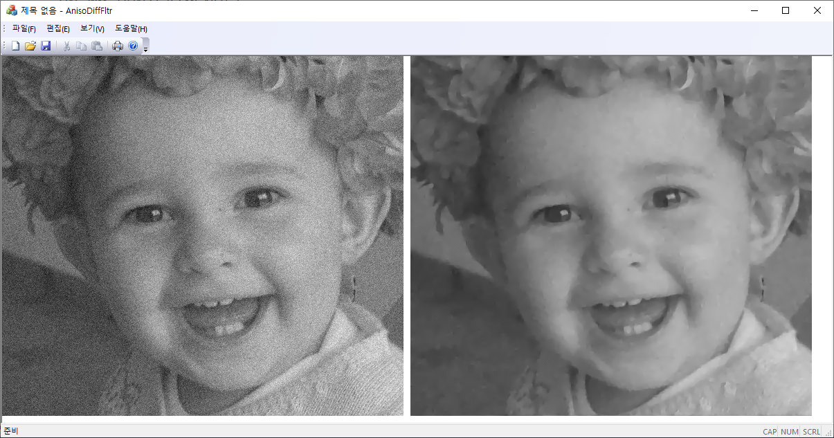
int BilateralFilter(BYTE *image, int width, int height, 
    double sigmas, double sigmar, int ksize, BYTE* out) {
    //const double sigmas = 1.7;
    //const double sigmar = 50.;
    double sigmas_sq = sigmas * sigmas;
    double sigmar_sq = sigmar * sigmar;
    //const int ksize = 7;
    const int hksz = ksize / 2;
    ksize = hksz * 2 + 1;
    std::vector<double> smooth(width * height, 0);
    // LUT for spatial gaussian;
    std::vector<double> spaceKer(ksize * ksize, 0);
    for (int j = -hksz, pos = 0; j <= hksz; j++) 
        for (int i = -hksz; i <= hksz; i++) 
            spaceKer[pos++] = exp(- 0.5 * double(i * i + j * j)/ sigmas_sq); 
    // LUT for image similarity gaussian;
    double pixelKer[256];
    for (int i = 0; i < 256; i++)
        pixelKer[i] = exp(- 0.5 * double(i * i) / sigmar_sq);

    for (int y = 0, imgpos = 0; y < height; y++) {
        int top = y - hksz;
        int bot = y + hksz;
        for (int x = 0; x < width; x++) {
            int left = x - hksz;
            int right = x + hksz;
            // convolution;
            double wsum = 0;
            double fsum = 0; 	
            int refVal = image[imgpos];
            for (int yy = top, kpos = 0; yy <= bot; yy++) {
                for (int xx = left; xx <= right; xx++) {
                    // check whether the kernel rect is inside the image;
                    if ((yy >= 0) && (yy < height) && (xx >= 0) && (xx < width)) {
                        int curVal = image[yy * width + xx];
                        int idiff = curVal - refVal;
                        double weight = spaceKer[kpos] * pixelKer[abs(idiff)];
                        wsum += weight;
                        fsum += weight * curVal;
                    }
                    kpos++;
                }
            }
            smooth[imgpos++] = fsum / wsum;
        }
    }

    for (int k = smooth.size(); k-- > 0;) {
        int a = int(smooth[k]);
        out[k] = a < 0 ? 0: a > 255 ? 255: a;
    }
    return 1;
}