Geometry & Recognition

일정한 간격 $h$마다 샘플링된 데이터 $\{(x_k,f_k)\}$를 이용해서 이들 데이터를 표현하는 spline를 구해보자. spline은 주어진 샘플링 데이터을 통과할 필요는 없으므로 일반적으로 interpolation 함수는 아니다. 이 spline은 샘플링 데이터와 kernel이라고 불리는 함수의 convolution 형태로 표현할 수 있다.

$$g(x)=\sum _k{f}_{k}K\left(\frac{x-x_k}{h}\right)$$

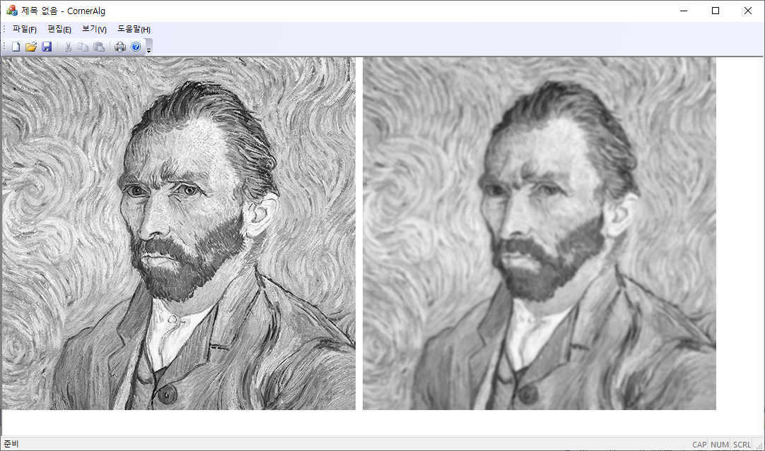
이미지의 resampling 과정에서 spline를 이용하는데 이때 사용 가능한 kernel의 형태와 그 효과를 간단히 알아보자.

3차 spline kernel은 중심을 기준으로 반지름이 2인 영역 $(-2,1),(-1,0),(0,1),(1,2)$에서만  0이 아닌 piecewise 삼차함수다. 그리고 이 함수는 우함수의 특성을 갖는다. 따라서 가능한 형태는

$$K(s)=\{\begin{array}{cc}{A}_1|s{|}^3+B_1|s{|}^2+C_1|s|+D_1& |s|<1\\ A_2|s{|}^3+B_2|s{|}^2+C_2|s|+D_2& 1\le |s|<2\\ 0& \text{otherwise}\end{array}$$처럼 쓸 수 있다. 계수를 완전히 결정하기 위해서는 8개의 조건이 필요한다. 우선 우함수이므로 원점에서 미분값이 제대로 정의되려면 $$C_1=0$$도 만족해야 한다, 그리고 각 node에서 연속성을 요구하면

$$\begin{array}{rl}s=1^{\pm }:& A_1+B_1+D_1=A_2+B_2+C_2+D_2\\ s=2^{\pm }:& 8A_2+4B_2+2C_2+D_2=0\end{array}$$ 임을 알 수 있다. 또한 각 node에서 부드럽게 연결되기 위해서 1차 도함수가 연속적임을 요구하면

$$\begin{array}{rl}s=1^{\pm }:& 3A_1+2B_1=3A_2+2B_2+C_2\end{array}$$

그리고 샘플링된 데이터가 모두 같은 경우 보간함수도 상수함수가 되는 것이 타당하므로

$$g(x)=\sum _{k}K\left(\frac{x-x_k}{h}\right)=1\text{if}\mathrm{\forall }{f}_j=1$$

을 만족시켜야 한다. $x_j<x<x_{j+1}$일 때 $x=x_j+sh,(0<s<1)$로 쓸 수 있고, kernel이 반지름이 2인  support를 가지므로 

$$g(x)=K(s+1)+K(s)+K(s-1)+K(s-2)=1$$

임을 알 수 있다. 위에서 주어진 $K(s)$을 대입해서 정리하면 다음과 같은 항등식을 얻는다.

$$\begin{gathered} -1+A_1+9A_2+B_1+5B_2+3C_2+2D_1+2D_2 \\ +(-3A_1-9A_2-2B_1-2B_2)s+(3A_1+9A_2+2B_1+2B_2)s^2=0 \end{gathered}$$

이 항등식의 계수가 0이 되어야 한다는 사실에서 2 개의 추가 조건을 얻으므로 총 8개 계수 중 2개가 미결정 free parameter로 남는다. 보통 이 두 계수는 $D_1=1-B/3$,  $D_2=4C+4B/3$처럼 매개화한다. 이 경우 kernel 함수는

$$K(s)=\frac{1}{6}\{\begin{array}{cc}(12-9B-6C)|s{|}^3+(-18+12B+6C)|s{|}^2+(6-2B)& |s|<1\\ (-B-6C)|s{|}^3+(6B+30C)|s{|}^2+(-12B-48C)|s|+(8B+24C)& 1\le |s|<2\\ 0& \text{otherwise}\end{array}$$

따라서 cubic spline kernel은 두 개의 파라미터 (B,C)에 의해서 정해진다. 또한 kernel 함수의 적분은 $B,C$에 상관없이 항상 1이어서 총 가중치의 합이 1임이 자동으로 보증된다.

$${\int }_{-\mathrm{\infty }}^{\mathrm{\infty }}K(s)ds=1$$

이 중에는 이미지의 resampling에서 많이 사용되는 커널도 있는데, 잘 알려진 경우를 보면

$$\begin{array}{cc}(B,C)=(0,1)& \text{Cardinal spline}\\ (B,C)=(0,1/2)& \text{Catmull-Rom spline }\\ (B,C)=(0,3/4)& \text{used in photoshop}\\ (B,C)=(1/3,1/3)& \text{ Mitchell-Netravali spline}\\ (B,C)=(1,0)& \text{B-spline}\end{array}$$

$B=0$인 경우는 $s=0$일 때 1이고, $|s|=1,2$일 0이므로 interpolation kernel($K(i-j)={\delta }_{ij}$)에 해당한다. 그리고 $B=0,C=1/2$인 경우인 Catmul-Rom spline은 node에서 2차 도함수까지도 연속이므로 샘플링 데이터를 생성한 원 아날로그 함수에 $O(h^3)$이내에서 가장 유사하게 근사함을 보일 수도 있다.

// Mitchell Netravali Reconstruction Filter
// B = 0    C = 0   - Hermite B-Spline interpolator 
// B = 0,   C = 1/2 - Catmull-Rom spline
// B = 1/3, C = 1/3 - Mitchell Netravali spline
// B = 1,   C = 0   - cubic B-spline
double MitchellNetravali(double x, double B, double C) {
    x = fabs(x);
    if (x >= 2) return 0;
    double xx = x*x;
    if (x >= 1) return ((-B - 6*C)*xx*x 
                + (6*B + 30*C)*xx + (-12*B - 48*C)*x 
                + (8*B + 24*C))/6;
    if (x < 1) return ((12 - 9*B - 6*C)*xx*x +
        (-18 + 12*B + 6*C) * xx + (6 - 2*B))/6;
}

일반적인 conic section 피팅은 주어진 데이터 $\{(x_i,y_i)\}$를 가장 잘 기술하는 이차식

$$F(x,y)=a{x}^2+bxy+c{y}^2+dx+ey+f=0$$

의 계수 ${\mathbf{u}}^{\mathbf{T}}=(a,b,c,d,e,f)$을 찾는 문제이다. 이 conic section이 타원이기 위해서는 2차항의 계수 사이에 다음과 같은 조건을 만족해야 한다.

$$\text{ellipse constraint:}ac-b^2/4>0$$

그리고 얼마나 잘 피팅되었난가에 척도가 필요한데 여기서는 주어진 데이터의 대수적 거리 $F(x,y)$을 이용하자. 주어진 점이 타원 위의 점이면 이 값은 정확히 0이 된다. 물론 주어진 점에서 타원까지의 거리를 사용할 수도 있으나 이는 훨씬 복잡한 문제가 된다.  따라서 해결해야 하는 문제는

$$\begin{array}{c}L=\sum _i{(a{x}_i^2+b{x}_i{y}_i+c{y}_i^2+d{x}_i+e{y}_i+f)}^2-\lambda (4ac-b^2-1)\\ ={\left|\left(\begin{array}{cccccc}{x}_0^2& x_0{y}_0& y_0^2& x_0& y_0& 1\\ x_1^2& x_1{y}_1& y_1^2& x_1& y_1& 1\\ x_2^2& x_2{y}_2& y_2^2& x_2& y_2& 1\\ & & ⋮\end{array}\right)\left(\begin{array}{c}a\\ b\\ c\\ d\\ e\\ f\end{array}\right)\right|}^2-\lambda ({\mathbf{u}}^{\mathbf{T}}\left(\begin{array}{cccccc}0& 0& 2& 0& 0& 0\\ 0& -1& 0& 0& 0& 0\\ 2& 0& 0& 0& 0& 0\\ 0& 0& 0& 0& 0& 0\\ 0& 0& 0& 0& 0& 0\\ 0& 0& 0& 0& 0& 0& \end{array}\right)\mathbf{u}\mathbf{-}\mathbf{1})\\ ={\mathbf{u}}^{\mathbf{T}}{\mathbf{D}}^{\mathbf{T}}\mathbf{D}\mathbf{u}\mathbf{-}\lambda \mathbf{(}{\mathbf{u}}^{\mathbf{T}}\mathbf{C}\mathbf{u}\mathbf{-}\mathbf{1}\mathbf{)}\\ ={\mathbf{u}}^{\mathbf{T}}\mathbf{S}\mathbf{u}\mathbf{-}\lambda \mathbf{(}{\mathbf{u}}^{\mathbf{T}}\mathbf{C}\mathbf{u}\mathbf{-}\mathbf{1}\mathbf{)}\end{array}$$

을 최소화시키는 계수 벡터 $\mathbf{u}$를 찾는 것이다. 여기서 제한조건으로 $4ac-b^2=1={\mathbf{u}}^{\mathbf{T}}\mathbf{C}\mathbf{u}$로 설정했다. 

${\mathbf{u}}^{\mathbf{T}}$에 대해서 미분을 하면 

$$\frac{\partial L}{\partial {\mathbf{u}}^{\mathbf{T}}}=\mathbf{S}\mathbf{u}\mathbf{-}\lambda \mathbf{C}\mathbf{u}\mathbf{=}\mathbf{0}$$

즉, 주어진 제한조건 $4ac-b^2=1$하에서 대수적 거리를 최소화시키는 타원방정식의 계수 $\mathbf{u}$를 구하는 문제는 scattering matrix $\mathbf{S}\mathbf{=}{\mathbf{D}}^{\mathbf{T}}\mathbf{D}$에 대한 일반화된 고유값 문제로 환원이 된다.

$$\begin{gathered} \mathbf{S}\mathbf{u}\mathbf{=}\lambda \mathbf{C}\mathbf{u} \\ {\mathbf{u}}^{\mathbf{T}}\mathbf{C}\mathbf{u}\mathbf{=}\mathbf{1} \end{gathered}$$

이 문제의 풀이는 직전의 포스팅에서 다른 바 있는데 $\mathbf{S}$의 제곱근 행렬 $\mathbf{Q}\mathbf{=}{\mathbf{S}}^{\mathbf{1}\mathbf{/}\mathbf{2}}$를 이용하면 된다. 주어진 고유값 $\lambda$와 고유벡터 $\mathbf{u}$가 구해지면 대수적 거리는 $${\mathbf{u}}^{\mathbf{T}}\mathbf{S}\mathbf{u}\mathbf{=}\lambda$$

이므로 이를 최소화시키기 위해서는 양의 값을 갖는 고유값 중에 최소에 해당하는 고유벡터를 고르면 된다. 그런데 고유값 $\lambda$의 부호별 개수는 $\mathbf{C}$의 고유값 부호별 개수와 동일함을 보일 수 있는데 (Sylverster's law of inertia),  $\mathbf{C}$의 고유값이 $\{-2,-1,2,0,0,0\}$이므로 $\lambda >0$인 고유값은 1개 뿐임을 알 수 있다. 따라서 $\mathbf{S}\mathbf{u}\mathbf{=}\lambda \mathbf{C}\mathbf{u}$를 풀어서 얻은  유일한 양의 고유값에 해당하는 고유벡터가 원하는 답이 된다.

https://kipl.tistory.com/370

https://kipl.tistory.com/565

 Ref: https://www.microsoft.com/en-us/research/wp-content/uploads/2016/02/ellipse-pami.pdf

double FitEllipse(std::vector<CPoint>& points, double einfo[6] ) {     
    if ( points.size() < 6 ) return -1;
    double eigvals[6];
    std::vector<double> D(6 * points.size());
    double S[36];/*  S = ~D * D  */
    double C[36];
    double EIGV[36];/* R^T; transposed orthogonal matrix;*/

    double offx = 0, offy = 0;
    /* shift all points to zero */
    for(int i = points.size(); i--> 0; ) {	
        offx += points[i].x;
        offy += points[i].y;        	
    }
    offx /= points.size(); 
    offy /= points.size();

    /* for the sake of numerical stability, scale down to [-1:1];*/
    double smax = points[0].x, smin = points[0].y;
    for (int i = points.size(); i-->1; ) {
        smax = max(smax, max(points[i].x, points[i].y));
        smin = min(smin, min(points[i].x, points[i].y));
    }
    double scale = smax - smin; 
    double invscale = 1 / scale;
    /* ax^2 + bxy + cy^2 + dx + ey + f = 0*/
    /* fill D matrix rows as (x*x, x*y, y*y, x, y, 1 ) */
    for(int i = points.size(); i--> 0; ) {	
        double x = points[i].x - offx; x *= invscale; 
        double y = points[i].y - offy; y *= invscale;
        D[i*6 + 0] = x*x; D[i*6 + 1] = x*y;
        D[i*6 + 2] = y*y; D[i*6 + 3] = x;
        D[i*6 + 4] = y;   D[i*6 + 5] = 1;		
    }			

    /* scattering matrix: S = ~D * D (6x6)*/
    for (int i = 0; i < 6; i++) 
        for (int j = i; j < 6; j++) { /*upper triangle;*/
            double s = 0;
            for (int k = points.size(); k-- > 0; ) 
                s += D[k*6 + i] * D[k*6 + j];
            S[i*6 + j] = s;
        }
    for (int i = 1; i < 6; i++) /*lower triangle;*/
        for (int j = 0; j < i; j++) 	
            S[i*6 + j] = S[j*6 + i] ;
    
    /* fill constraint matrix C */
    for (int i = 0; i < 36 ; i++ ) C[i] = 0;
    C[12] =  2 ;//2x0 
    C[2 ] =  2 ;//0x2 
    C[7 ] = -1 ;//1x1

    /* find eigenvalues/vectors of scattering matrix; */
    double RT[36];	/* each row contains eigenvector; */
    JacobiEigens ( S, RT, eigvals, 6, 0 );
    /* create R and INVQ;*/
    double R[36];
    for (int i = 0; i < 6 ; i++) {
        eigvals[i] = sqrt(eigvals[i]);
        for ( int k = 0; k < 6; k++ ) {
            R[k*6 + i] = RT[i*6 + k];  /* R = orthogonal mat = transpose(RT);*/
            RT[i*6 + k] /= eigvals[i]; /* RT /= sqrt(eigenvalue) row-wise)*/
        }
    }
    /* create INVQ=R*(1/sqrt(eigenval))*RT;*/
    double INVQ[36];
    _MatrixMul(R, RT, 6, INVQ);

    /* create matrix INVQ*C*INVQ */
    double TMP1[36], TMP2[36];
    _MatrixMul(INVQ, C, 6, TMP1 );
    _MatrixMul(TMP1, INVQ, 6, TMP2 );
    
    /* find eigenvalues and vectors of INVQ*C*INVQ:*/
    JacobiEigens ( TMP2, EIGV, eigvals, 6, 0 );
    /* eigvals stores eigenvalues in descending order of abs(eigvals);*/
    /* search for a unique positive eigenvalue;*/
    int index = -1, count = 0;
    for (int i = 0 ; i < 3; i++ ) {
        if (eigvals[i] > 0) {
            index = i; // break;
            count++;
        }
    }
    /* only 3 eigenvalues must be non-zero 
    ** and only one of them must be positive;*/
    if ((count != 1) || (index == -1)) 
        return -1;
     
    /* eigenvector what we want: u = INVQ * v */
    double u[6]; 
    double *vec = &EIGV[index*6];
    for (int i = 0; i < 6 ; i++) {
        double s = 0;
        for (int k = 0; k < 6; k++) s += INVQ[i*6 + k] * vec[k];
        u[i] = s;
    }
    /* extract shape infos;*/
    PoseEllipse(u, einfo);
    /* recover original scale; center(0,1) and radii(2,3)*/
    for (int i = 0; i < 4; i++) einfo[i] *= scale;
    /* recover center */
    einfo[0] += offx; 
    einfo[1] += offy;
    return FitError(points, offx, offy, scale, u);
};

$$\begin{array}{c}BF[I{]}_{\mathbf{p}}=\frac{1}{W_{\mathbf{p}}}\sum _{\mathbf{q}\in S}{G}_{{\sigma }_s}(||\mathbf{p}-\mathbf{q}||)G_{{\sigma }_r}(|I_{\mathbf{p}}-I_{\mathbf{q}}|)I_{\mathbf{q}}\\ W_{\mathbf{p}}=\sum _{\mathbf{q}\in S}{G}_{{\sigma }_s}(||\mathbf{p}-\mathbf{q}||)G_{{\sigma }_r}(|I_{\mathbf{p}}-I_{\mathbf{q}}|)\\ G_{\sigma }(\mathbf{r})=e^{-||\mathbf{r}\mathbf{|}{\mathbf{|}}^{\mathbf{2}}\mathbf{/}\mathbf{2}{\sigma }^{\mathbf{2}}}\end{array}$$

// sigmar controls the intensity range that is smoothed out. 
// Higher values will lead to larger regions being smoothed out. 
// The sigmar value should be selected with the dynamic range of the image pixel values in mind.
// sigmas controls smoothing factor. Higher values will lead to more smoothing.
// convolution through using lookup tables.
int BilateralFilter(BYTE *image, int width, int height, 
    double sigmas, double sigmar, int ksize, BYTE* out) {
    //const double sigmas = 1.7;
    //const double sigmar = 50.;
    double sigmas_sq = sigmas * sigmas;
    double sigmar_sq = sigmar * sigmar;
    //const int ksize = 7;
    const int hksz = ksize / 2;
    ksize = hksz * 2 + 1;
    std::vector<double> smooth(width * height, 0);
    // LUT for spatial gaussian;
    std::vector<double> spaceKer(ksize * ksize, 0);
    for (int j = -hksz, pos = 0; j <= hksz; j++) 
        for (int i = -hksz; i <= hksz; i++) 
            spaceKer[pos++] = exp(- 0.5 * double(i * i + j * j)/ sigmas_sq); 
    // LUT for image similarity gaussian;
    double pixelKer[256];
    for (int i = 0; i < 256; i++)
        pixelKer[i] = exp(- 0.5 * double(i * i) / sigmar_sq);

    for (int y = 0, imgpos = 0; y < height; y++) {
        int top = y - hksz;
        int bot = y + hksz;
        for (int x = 0; x < width; x++) {
            int left = x - hksz;
            int right = x + hksz;
            // convolution;
            double wsum = 0;
            double fsum = 0; 	
            int refVal = image[imgpos];
            for (int yy = top, kpos = 0; yy <= bot; yy++) {
                for (int xx = left; xx <= right; xx++) {
                    // check whether the kernel rect is inside the image;
                    if ((yy >= 0) && (yy < height) && (xx >= 0) && (xx < width)) {
                        int curVal = image[yy * width + xx];
                        int idiff = curVal - refVal;
                        double weight = spaceKer[kpos] * pixelKer[abs(idiff)];
                        wsum += weight;
                        fsum += weight * curVal;
                    }
                    kpos++;
                }
            }
            smooth[imgpos++] = fsum / wsum;
        }
    }

    for (int k = smooth.size(); k-- > 0;) {
        int a = int(smooth[k]);
        out[k] = a < 0 ? 0: a > 255 ? 255: a;
    }
    return 1;
}