It is well known that the convex hull of a set of n points in the (Euclidean) plane can be found by an algorithm having worst-case complexity O(n log n). In this note we give a short linear algorithm for finding the convex hull in the, case that the (ordered) set of points from the vertices of a simple (i.e., non-self-intersecting) polygon.
http://deepblue.lib.umich.edu/bitstream/2027.42/7588/5/bam3301.0001.001.pdf We present space-efficient algorithms for computing the convex hull of a simple polygonal line in-place, in linear time. It turns out that the problem is as hard as stable partition, i.e., if there were a truly simple solution then stable partition would also have a truly simple solution, and vice versa. Nevertheless, we present a simple self-contained solution that uses O(log n) space, and indicate how to improve it to O(1) space with the same techniques used for stable partition. If the points inside the convex hull can be discarded, then there is a truly simple solution that uses a single call to stable partition, and even that call can be spared if only extreme points are desired (and not their order). If the polygonal line is closed, then the problem admits a very simple solution which does not call for stable partitioning at all.
The Savitzky–Golay method essentially performs a local polynomial regression (of degree $k$) on a series of values (of at least $k+1$ points which are treated as being equally spaced in the series) to determine the smoothed value for each point.
Savitzky–Golay 필터는 일정한 간격으로 주어진 데이터들이 있을 때(이들 데이터는 원래의 정보와 노이즈를 같이 포함한다), 각각의 점에서 주변의 점들을 가장 잘 피팅하는 $k$-차의 다항식을 최소자승법으로 찾아서 그 지점에서의 출력값을 결정하는 필터이다. 이 필터는 주어진 데이터에서의 극대나 극소, 또는 봉우리의 폭을 상대적으로 잘 보존한다.(주변 점들에 동등한 가중치를 주는 Moving Average Filter와 비교해 볼 수 있다).
위에서 계수 $a_0$, $a_1$, $a_2$를 결정하는 방정식은 행렬로 정리하면 아래의 식과 같이 표현할 수 있다.
좌변의 5행 3열 행렬을 $\mathbf{A}$, ${\mathbf{a}}=[a_0, a_1, a_2]^T$, ${\mathbf{d}}=[d_0, d_1, d_2, d_3, d_4]^T$로 놓으면, 이 행렬방정식은 $\mathbf{ A.a = d}$ 형태로 쓸 수 있다. $\mathbf{A}$가 정방행렬이 아니므로 역행렬을 바로 구할 수 없지만, $|\mathbf{ A \cdot a - d} |^2$을 최소로 하는 최소제곱해는 $$\bf (A^T\cdot A)\cdot a = A^T \cdot d$$를 만족시켜야 하므로
$$\bf a = (A^T\cdot A)^{-1} \cdot (A^T \cdot d)$$로 주어짐을 알 수 있다.
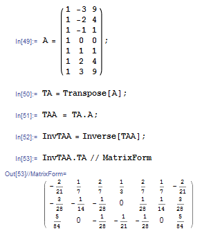
이 식은 임의의 $k$-차 다항식을 이용한 경우에도 사용할 수 있다. 이 경우 행렬 $\bf A^T \cdot A$는 $(k+1)\times (k+1)$의 대칭행렬이 된다.행렬 $\bf A$는 다항식의 찻수와 피팅에 사용이 될 데이터의 구간의 크기가 주어지면 정해지므로, 윗 식에서 $({\bf A}^T\cdot {\bf A})^{-1}\cdot {\bf A}^T$의 첫 행 ($a_0$을 $d$로 표현하는 식의 계수들)을 구하면 코드 내에서 결과를 lookup table로 만들어서 사용할 수 있다. 아래 표는 mathematica 를 이용해서 윈도 크기가 7 (7개 점)인 경우 2차 다항식을 사용할 때 계수를 구하는 과정이다.
2차 다항식일 때, 같은 방식으로 다양한 윈도 크기에 따른 계수를 구할 수 있다. *크기($n$)에 따른 필터값 결정계수 (중앙에 대해 좌우대칭이다);
Retinex 알고리즘은 영상의 contrast를 향상하거나, sharpness를 증진시킬 때 많이 사용한다. 또 픽셀 값의 dynamic range가 큰 경우에 이것을 압축시켜 영상 데이터 전송에 따른 병목 현상의 해소에 이용할 수 있다. Retinex 알고리즘의 기본 원리는 입력 영상에 들어있는 배경 성분을 제거하는 것이다.
1. 배경 영상은 입력 영상의 평균적인 영상로 생각할 수 있는데, 이것은 적당한 스케일(필터 사이즈)의 가우시안 필터를 적용하여서 얻을 수 있다. 이 필터를 적용하면 입력 영상에서 필터 사이즈보다 작은 스케일은 무시하는 효과를 준다. 2. 입력 영상의 반사 성분(배경 조명에 무관한)은 입력 영상을 앞서 구한 배경 영상으로 나누면 된다 3. Retinex 출력은 이 반사 성분에 로그 값을 취한 것이다. 로그를 취함으로써 반사 성분이 분포 범위(=dynamic range)를 압축하는 효과를 얻는다.
이처럼 하나의 스케일에 대해서 적용하는 경우를 SSR(single-scale retinex) 알고리즘이라고 한다. 컬러 영상의 경우에는 각각의 RGB 채널에 대해 알고리즘을 적용하면 된다.
Retinex 영상을 구할 때 하나의 스케일이 아니라 다중 스케일에 대해서 적용한 retinex 영상을 적절한 가중치($\omega_\sigma$)를 주어서 더한 결과를 출력 영상으로 사용할 수 있다. 이 경우가 MSR(multi-scale retinex) 알고리즘이다. $$R_{MSR}(x,y) = \sum_{\sigma\in scales} \omega_{\sigma} R_{SSR}(x,y;\sigma) $$
이렇게 얻은 Retinex 출력 영상은 적당한 offset과 stretching을 하여서 픽셀 값이 [0,255] 구간에 있게 조절한다. 이 과정은 Retinex 출력 영상 픽셀의 평균값과 편차를 구하여 해결한다.
컬러 영상의 경우에 Retinex 출력 영상은 전체적으로 그레이화 되는 경향이 있어서 이것을 보완하기 위해서 아래의 추가적인 처리 과정을 더 거친다. $$ {\tilde R}_{MSR}^{red}(x,y)=\log \left(\frac{C I_{red}}{ I_{red}+I_{green}+I_{blue}} \right) R_{MSR}^{red}(x,y)$$ $$ {\tilde R}_{MSR}^{grren}(x,y)=\log \left(\frac{CI_{green}}{ I_{red}+I_{green}+I_{blue}} \right) R_{MSR}^{green}(x,y)$$ $$ {\tilde R}_{MSR}^{blue}(x,y)=\log \left(\frac{C I_{blue}}{I_{red} +I_{green}+I_{blue}} \right) R_{MSR}^{blue}(x,y)$$
여기서, $C$는 상수이고, $I_{red}, I_{green}, I_{blue}$는 입력 영상의 RGB-채널이다.
*그레이 이미지 처리 결과:
*구현 코드는 다음을 참고: 그레이: http://kipl.tistory.com/33 컬러: http://blog.naver.com/helloktk/80039132534 * 기술적으로 log를 취하므로 입력 영상에 +1을 더해서 log(0)이 나오는 것을 방지해야 한다. * convolution 된 영상도 1보다 작은 경우에 1로 만들어야 한다. * 스케일이 큰 경우에 필터 사이즈가 매우 크므로 효과적인 convolution 알고리즘을 생각해야 한다. 보통 recursive 필터링을 하여서 빠르게 convolution결과를 얻는다.
각각 200개의 점들로 이루어진 8개의 2차원 가우시안 군집을 무작위로 만들고, 이를 kmeans 알고리즘을 써서 8개로 분할하였다. 아래의 시뮬레이션은 이 정보를 초기 조건으로 하여서 Gaussian Mixture Model (GMM)에 적용한 결과이다. 두 개의 군집에 대해서 kmeans 결과와 GMM의 결과가 서로 많이 차이가 남을 보여준다.
코드 추가: 2010.02.23
struct Data2d {
    double x, y ;
    int id ;
    Data2d() { };
    Data2d(double x, double y) : x(x), y(y), id(-1) { }
};
struct Gauss2d {
    double cov[4];
    double mx, my ; //mean ;
    double mix;
    //
    double nfactor; //1/(2 * Pi * sqrt(det));
    double det;     //det(cov)
    double icov[4];
    void   prepare();
    //
    double pdf(double x, double y);
} ;
void Gauss2d::prepare() {
    // det(cov);
    det = cov[0] * cov[3] - cov[1] * cov[2];
    if (det < 1e-10) {
        AfxMessageBox("not converging");
        return ;
    };
    nfactor = 1. / (2. * MPI * sqrt(det)) ;
    //inv(cov);
    icov[0] =  cov[3] / det;
    icov[1] = -cov[1] / det;
    icov[2] = -cov[2] / det;
    icov[3] =  cov[0] / det;
}
double Gauss2d::pdf(double x, double y) {
    x -= mx ;
    y -= my ;
    double a = x * (icov[0] * x + icov[1] * y) +
               y * (icov[2] * x + icov[3] * y);
    return (nfactor * exp(-0.5 * a));
};
void init_classes(std::vector<Data2d>& data, std::vector<Gauss2d>& classes) {
    /*
    for (int i = 0; i < classes.size(); i++) {
        Gauss2d& cls = classes[i] ;
        cls.cov[0] = 10 + 50 * rand() / double(RAND_MAX);
        cls.cov[1] = 0;
        cls.cov[2] = 0;
        cls.cov[3] = 10 + 50 * rand() / double(RAND_MAX);
        cls.mx = 100 + 300 * rand() / double(RAND_MAX);
        cls.my = 100 + 300 * rand() / double(RAND_MAX);
        cls.mix = 1;
    }
    */
    KMeans(data, classes);
    //use kmeans to locate initial positions;
}
void test_step(std::vector<Data2d>& data,
               std::vector<Gauss2d>& classes,
               std::vector<std::vector<double> >& prob_cls)
{
    //E-step ;
    for (int k = 0; k < classes.size(); k++) {
        Gauss2d& cls = classes[k];
        cls.prepare();
        //
        for (int i = 0; i < data.size(); i++) {
            prob_cls[i][k] = cls.mix * cls.pdf(data[i].x, data[i].y);
        };
    }
    // normalize-->임의의 데이터는 각 어떤 클레스에 속할 활률의 합=1;
    for (int i = 0; i < data.size(); i++) {
        double s = 0;
        int bc = 0; double bp = 0;  // to determine membership(debug);
        for (int k = 0; k < classes.size(); ++k) {
            s += prob_cls[i][k];
            // find maximum posterior for each data;
            if (bp < prob_cls[i][k]) {
                bp = prob_cls[i][k] ;
                bc = k ;
            };
        }
        data[i].id = bc;
        // normalize to 1;
        for (int k = 0; k < classes.size(); ++k)
            prob_cls[i][k] /= s;
    }
    //M-step;
    for (int k = 0; k < classes.size(); k++) {
        Gauss2d & cls = classes[k];
        //get mean;
        double meanx    = 0;
        double meany    = 0;
        double marginal = 0;
        for (int i = 0; i < data.size(); i++) {
            meanx    += prob_cls[i][k] * data[i].x ;
            meany    += prob_cls[i][k] * data[i].y ;
            marginal += prob_cls[i][k];
        };
        cls.mx = meanx = meanx / marginal ;
        cls.my = meany = meany / marginal ;
        // get mixing;
        cls.mix = marginal / classes.size();
        // get stdev;
        double sxx = 0, syy = 0, sxy = 0;
        for (int i = 0; i < data.size(); i++) {
            double dx = data[i].x - meanx ;
            double dy = data[i].y - meany ;
            sxx += prob_cls[i][k] * dx * dx ;
            syy += prob_cls[i][k] * dy * dy ;
            sxy += prob_cls[i][k] * dx * dy ;
        };
        //set covariance;
        cls.cov[0] = sxx / marginal;
        cls.cov[1] = sxy / marginal;
        cls.cov[3] = syy / marginal;
        cls.cov[2] = cls.cov[1]; //symmetric;
    }
}
void test() {
    int max_iter = 100;
    int nclass = 8;
    int ndata = 500;
    std::vector<Gauss2d> classes(nclass);
    std::vector<Data2d> data(ndata);
    // prepare posterior space;
    std::vector<std::vector<double> > prob_cls;
    for (int i = 0; i < data.size(); ++i) {
        prob_cls.push_back(std::vector<double>(classes.size()));
    } ;
   // generate data...
   ..................................
    //init_classes
    init_classes(data, classes) ;

    int iter = 0;
    do {
        iter++;
        test_step(data, classes, prob_cls);
    } while (iter < max_iter) ;
};