구간 $[a=t_0, ...t_{n-1}=b]$에서 일정한 간격(꼭 일정한 간격일 필요는 없지만 여기서는 1로 선택함)으로 샘플링된 데이터 $\{ f_0, ...f_{n-1} \}$이 있다. $n-1$ 개의 각 구간에서 데이터를 보간하는 삼차다항식 함수 모임 $$S(t)= \{S_j (t)| t_j \le t <t_{j+1} , ~~j=0,1,2...,n-2 \} $$을 찾아보자. 전체 구간에서 연속적이고 충분히 부드럽게 연결되기 위해서는 우선 각 node에서 연속이어야 하고, 또한 1차 도함수와 2차 도함수도 연속이 되어야 한다. 물론 각 node에서는 샘플링된 데이터값을 가져야 한다.
\begin{align} (a) ~~& S(t_j) = f_j \\ (b)~~& S_{j+1}(t_{j+1}) = S_j( t_{j+1}) \\ (c)~~& S'_{j+1}(t_{j+1}) = S'_j(t_{j+1}) \\ (d)~~& S''_{j+1}(t_{j+1}) = S''_{j}(t_{j+1}) \end{align}
$n-1$개 구간에서 각각 정의된 3차 함수를 결정하려면 $4 \times (n-1)$개의 조건이 필요하다. (a)에서 $n$개, (b), (c), (d)에서 $3\times (n-2)$개의 조건이 나오므로 총 $n+3\times(n-2)=4n-6$개의 조건만 생긴다. 삼차식을 완전히 결정하기 위해서는 2개의 추가적인 조건을 부여해야 하는데 보통 양끝에서 2차 도함수값을 0으로 하거나(natural boundary) 또는 양끝에서 도함수 값을 특정한 값으로 고정시킨다(clamped boundary). 여기서는 양끝의 2차 도함수를 0으로 한 natural cubic spline만 고려한다. 그리고 $S_j(t)$가 $n-2$개의 구간에 대해서만 정의되어 있지만, 끝점을 포하는 구간에서도 정의하자. 이 경우 $S_{n-1}(t), t\ge t_{n-1}$에 부여된 조건은 $t_{n-1}$에서 $S_{n-2}(t)$와 연속, 미분연속 그리고 2차 도함수가 0인 조건만 부여된다.
$j-$번째 구간의 삼차함수를
$$S_j(t) = a_j + b_j (t - t_j) + c_j (t-t_j)^2 + d_j (t - t_j)^3$$
로 쓰면 (a)에서
$$ S_j (t_j) = a_j = f_i,~~ j=0,1,..n-2$$
(b)에서
$$ a_{j+1} =a_j+ b_j + c_j +d_j,~~j=0,1,...,n-2$$
(c)에서
$$b_{j+1} = b_j + 2c_j+ 3d_j,~~j=0,1,...,n-2 $$
(d)에서
$$ c_{j+1} = c_j+ 3d_j,~~j=0,1,...,n-2$$
이므로 (b)와 (c)에서 $d_j$을 소거하면
$$ c_j = 3(a_{j+1}-a_j) -b_{j+1} - 2b_j$$
그리고 (a)에서 $$d_j = -2(a_{j+1}-a_j) + b_j + b_{j+1}$$ 이므로 $b_j$에 대해 정리하면 다음과 같은 점화식을 얻을 수 있다.
$$ b_{j+1} + 4b_j + b_{j-1}= 3(a_{j+1}- a_{j-1})=3(f_{j+1}-f_{j}),~~j=1,2,...,n-2$$
물론 $j=0$일 때는 (note, $S''_0(t_0) = 0 \to c_0=0$) $a_1 =a_0+b_0+d_0, b_1 = b_0 + 3d_0$이므로
$$ b_1 + 2b_0 = 3(f_1 - f_0) $$
$j=n-1$일 때 계수는 $S_{n-1}(t_{n-1}) = f_{n-1}$이고 $S''_{n-1}(t_{n-1} )=c_{n-1}=0$이므로 $$ 2b_{n-1} + b_{n-2} = 3(f_{n-1}-f_{n-2})$$
임을 알 수 있다. 따라서 계수를 구하는 과정은 $b_j~(j=0,...,n-1)$을 구하는 것으로 결정된다. 이를 행렬로 표현하면
$$ \begin{bmatrix} 2&1& \\1&4&1\\ &1&4&1 \\ & & & \cdots \\ &&&&1&4&1 \\ && & & & 1 &2 \end{bmatrix} \begin{bmatrix} b_0\\b_1\\ \vdots \\ b_{n-2} \\b_{n-1}\end{bmatrix}=\begin{bmatrix} 3(f_1-f_0) \\ 3(f_2-f_0) \\ \vdots \\ 3(f_{n-1}- f_{n-3}) \\3(f_{n-1} - f_{n-2}) \end{bmatrix}$$
와 같다. band 행렬은 upper triangle로 변환한 후 역치환과정을 거치면 쉽게 해를 구할 수 있다.
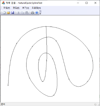
평면에서 주어진 점들을 보간하는 곡선은 이들 점을 표현하는 곡선의 매개변수를 일정한 간격으로 나누어서 샘플링된 결과로 취급하면, $x, y$ 성분에 대해서 각각 natural cubic spline를 구하여 얻을 수 있다.
struct Cubic {
    double a,b,c,d;  /* a + b*t + c*t^2 +d*t^3 */
    Cubic(double a_, double b_, double c_, double d_)
        : a(a_), b(b_), c(c_), d(d_) { }
    /* evaluate;*/
    double eval(double t) {
        return (((d*t) + c)*t + b)*t + a;
    }
};
void calcNaturalCubic(std::vector<double>& x, std::vector<Cubic>& Spline) {
    std::vector<double> gamma(x.size());
    std::vector<double> delta(x.size());
    std::vector<double> D(x.size());
    /* solve the banded equation:
    [2 1       ] [  D[0]]   [3(x[1]   - x[0])  ]
    |1 4 1     | |  D[1]|   |3(x[2]   - x[0])  |
    |  1 4 1   | | .    | = |      .           |
    |    ..... | | .    |   |      .           |
    |     1 4 1| | .    |   |3(x[N-1] - x[N-3])|
    [       1 2] [D[N-1]]   [3(x[N-1] - x[N-2])]
    ** make the banded matrix to an upper triangle;
    ** and then back sustitution. D[i] are the derivatives at the nodes.
    */
    const int n = x.size() - 1;  // note n != x.size()=N;
    // gamma;
    gamma[0] = 0.5;
    for (int i = 1; i < n; i++)
        gamma[i] = 1/(4-gamma[i-1]);
    gamma[n] = 1/(2-gamma[n-1]);
    // delta;
    delta[0] = 3*(x[1]-x[0])*gamma[0];
    for (int i = 1; i < n; i++)
        delta[i] = (3*(x[i+1]-x[i-1])-delta[i-1])*gamma[i];
    delta[n] = (3*(x[n]-x[n-1])-delta[n-1])*gamma[n];
    // D;
    D[n] = delta[n];
    for (int i = n; i-->0;)
        D[i] = delta[i] - gamma[i]*D[i+1];

    /* compute the coefficients;*/
    Spline.clear(); Spline.reserve(n);
    for (int i = 0; i < n; i++)
        Spline.push_back(Cubic(x[i], D[i], 3*(x[i+1]-x[i])-2*D[i]-D[i+1],
            2*(x[i]-x[i+1]) + D[i] + D[i+1])) ;
}
void NaturalCubicSpline(std::vector<CPoint>& points,
                        std::vector<CPoint>& curve) {
    curve.clear();
    if (points.size() < 2) return;
    std::vector<double> xp(points.size()), yp(points.size());
    for (int i = points.size(); i-->0;)
        xp[i] = points[i].x, yp[i] = points[i].y;

    std::vector<Cubic> splineX, splineY;
    calcNaturalCubic(xp, splineX);
    calcNaturalCubic(yp, splineY);
#define STEPS 12
    curve.reserve(splineX.size() * STEPS + 1);
    curve.push_back(CPoint(int(splineX[0].eval(0) + 0.5), int(splineY[0].eval(0) + 0.5)));
    for (int i = 0; i < splineX.size(); i++) {
        for (int j = 1; j <= STEPS; j++) {
            double t = double(j) / STEPS;
            curve.push_back(CPoint(int(splineX[i].eval(t)+0.5), int(splineY[i].eval(t)+0.5)));
        }
    }
}
'Computational Geometry' 카테고리의 다른 글
| Least Squares Bezier Fit (0) | 2024.04.05 |
|---|---|
| Why Cubic Splines? (9) | 2024.03.16 |
| Approximate Distance Between Ellipse and Point (0) | 2024.03.08 |
| Distance from a Point to an Ellipse (0) | 2024.03.06 |
| Data Fitting with B-Spline Curves (0) | 2021.04.30 |


