Geometry & Recognition

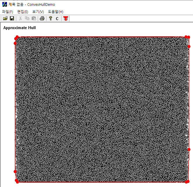
Fixed-point version: 선분 길이가 4096 픽셀 정도까지는 1-pixel 이내의 오차로 그려진다.

void DDALine(CPoint A, CPoint B) {
    const int mulfac = 4096; // 2^12 = 4096;
    int dx = B.x - A.x;
    int dy = B.y - A.y;
    int adx = dx < 0 ? -dx : dx;
    int ady = dy < 0 ? -dy : dy;
    int steps = adx < ady ? ady : adx;
    if (steps == 0) SetPixel(A.x, A.y); //single point;
    else {
        int curX = A.x * mulfac;      
        int curY = A.y * mulfac;
        dx = (dx * mulfac) / steps;
        dy = (dy * mulfac) / steps;
        while (steps-- >= 0) {
            SetPixel(curX / mulfac, curY / mulfac);
            curX += dx;
            curY += dy;
        }
    }
}

$$ \mathbf{C}(u) = \sum_{i=0}^{n} N_{i,p} (u) \mathbf{P}_i$$

where $N_{i, p}(u)$'s are B-spline basis functions of degree $p$, $n+1$ control points $\{\mathbf{P}_i\}$, and a knot vector $\mathbf{U}=(u_0, u_1, ..., u_m)$. Note, $m=n + p + 1$.

B-spline의 basis 함수 $N_{i, p}(t)$는 유한한 구간에서만 0이 아닌 값을 갖는(local support) 함수로 다음과 같은  recursion relation을 가진다:

\begin{align} N_{i,0}(t) &= \left\{ \begin{matrix} 1 & \mathrm{if} \quad u_i \leq x \lt u_{i+1} \\ 0 & \mathrm{otherwise} \end{matrix} \right. \quad \quad (0 \le i \le n+p), \\ N_{i,p}(t) &= \frac{t - u_i}{u_{i+p} - u_i} N_{i,p-1}(t) + \frac{u_{i+p+1} - t}{u_{i+p+1} - u_{i+1}} N_{i+1,p-1}(t).\end{align}

$N_{i,p}(t)$의 local support는 $[u_i, u_{i+p+1}]$로 주어진다.

일반적으로 knot vector가 특별한 구조를 가지지 않으면 B-spline곡선은 Bezier 곡선의 경우와 달리 처음과 끝 control 점을 통과하지 않는다(open B-spline). 처음과 끝점을 통과하도록 만들기 위해서는 knot 벡터의 시작 $(p+1)$개 성분이 같은 값을 갖고, 마지막 $(p+1)$개 성분도 같은 값을 갖도록 조정하면 된다(clamped B-spline):

$$clamped: u[0]=u[1]=...=u[p],...,u[n+1]=...=u[n+p]=u[n+p+1]$$

knot는 균일할 필요는 없지만, 균일한 경우는 보통

$$ u_i = \left\{ \begin{array} {rcl} 0 & , & 0 \le i \le p, \\ \frac{i-p}{n+1-p}&, & p+1\le i \le n \\ 1&,& n+1\le i \le n+p+1\end{array}\right.$$

로 선택한다. 

ref: ae.sharif.edu/~aerocad/curve%20modelling-B_Spline.pdf

clamped(black), open(blue)

// Note, p = degree;
void BSpline(int p, std::vector<CPoint>& control, int resolution, CDC *pDC) {
    int n = control.size() - 1;  ASSERT(n > 0);
    std::vector<double> u(n + p + 2);                // knot vector;
    calculateKnots(&u[0], n, p);                     // uniform knot;
    double delta = (u[n + p + 1] - u[0]) / (resolution - 1);  // parameter increment;
    CPoint Q;
    for (double t = u[0] ; t <= u[n+p+1]; t += delta) {
        calculatePoint(&u[0], n, p, t, &control[0], &Q);
        if (i == 0) pDC->MoveTo(Q);
        pDC->LineTo(Q);
    }
    pDC->LineTo(control[n]);
}
// de Boor Cox's algorithm;
double Blend(int i, int p, double *u, double t) {  
    if (p == 0) { // termination condition of recursion;
        if ((u[i] <= t) && (t < u[i+1]))        return 1;
        else                                    return 0;
    }
    else {
        double coef1, coef2;
        if (u[i+p] == u[i]) {
            if (t == u[i])  coef1 = 1;
            else            coef1 = 0;
        } 
        else                coef1 = (t - u[i]) / (u[i+p] - u[i]); 
        
        if (u[i+p+1] == u[i+1]) {
           if (t == u[i+1]) coef2 = 1;
           else             coef2 = 0;
        } 
        else                coef2 = (u[i+p+1] - t) / (u[i+p+1] - u[i+1]);
        return coef1 * Blend(i, p-1, u, t) + coef2 * Blend(i+1, p-1, u, t);
    }
}
// clamped b-spline knot vector; uniform example;
// u[0]=u[1]= ... =u[p],.....,u=[n+p-2]=u[n+p-1]=u[n+p]=u[n+p+1]
void calculateKnots(double *u, int n, int p) {
    int j = 0; 
    while (j <= p)     u[j++] = 0;                 // multiplicity = p+1;
    while (j <= n)     u[j++] = j - p;             // m = n+p+1;
    while (j <= n+p+1) u[j++] = n - p + 1;         // multiplicity = p+1;
}
void calculatePoint(double *u, int n, int p, double t, CPoint *control, CPoint *output) {
    double x = 0, y = 0;
    for (int i = 0; i <= n; i++) {
        double b = Blend(i, p, u, t);
        x += control[i].x * b;
        y += control[i].y * b;
    }
    output->x = int(x + 0.5);
    output->y = int(y + 0.5);
}

입력점들을 부드럽게 연결하는 베지어 곡선을 찾아보자. 입력점 사이 구간을 3차 베지어 곡선으로 표현하려면  4개의 컨트롤점이 필요한데, 최소자승법을 이용하지 않고 순차적인 3 입력점 $P_0, P_1, P_2$이 주어질 때 이를 이용해서 컨트롤 점을 구성한다.(따라서 베지어 곡선은 시작과 끝이 아닌 입력점을 일반적으로 통과하지 않는다)  $$C_0 = (P_0+P_1)/2,~~C_1 = (P_0 +5 P_1)/6,~~C_2 = (5P_1+  P_2)/6,~~C_3=(P_1+P_2)/2$$ 컨트롤점으로 하는 베지어 곡선은  $[P_0, P_1, P_2]$의 일부분을 표현한다. 이 과정은 다음 한 입력점을 포함시켜서 다시 반복을 하는데 이 떄  이전 베이어 곡선의 마지막 컨트롤점($C_2$)이 새로이 만들어지는 베지어 곡선의 시작점($C_0^\text{new}$)이 되므로 두 베지어 곡선은 부드럽게 연결이 된다. 입력점의 시작과 끝점은 베이어 곡선이 통과하도록 컨트롤점에 포함되게 설계한다.

$$\text{front}:~ C_0=P_0, ~~C_1 = (P_0+2P_1)/3$$

$$\text{back}:~C_2=(2P_1+P_2)/3, ~~C_3=P_3$$

그리고 주어진 베지어 곡선의 분할은 균일한 간격으로 하지 않고, 각각의 구간에서 베지어 곡선이 충분히 평탄하도록 분할해서 저장한다.

// test flatness of a bezier curve with control points {p1, c1, c2, p2};
bool FlatBezier(const double eps, 
                const CfPt& p1, const CfPt& c1, const CfPt& c2, const CfPt& p2) {
    CfPt U = c1 - (p1 * 2 + p2) / 3;
    CfPt V = c2 - (p1 + p2 * 2) / 3;
    double normU = hypot(U.x, U.y);
    double normV = hypot(V.x, V.y);
    return (3. * max(normU, normV) / 4.) <= eps;
}
// subdivision stage; De Casteljau's algorithm
void GetBezierPoints(const double eps, 
                     const CfPt &p1, const CfPt &c1, const CfPt &c2, const CfPt &p2,
                     std::vector<CfPt>& smoothed) {
    if (!FlatBezier(eps, p1, c1, c2, p2)) {
        // Subdivide the curve at t = 0.5
        // left;
        CfPt mid_segm = (p1  + c1 * 3 + c2 * 3 + p2) / 8.0; // = B(1/2);
        CfPt new_c1   = (p1 + c1) / 2.0;
        CfPt new_c2   = (p1 + c1 * 2 + c2) / 4.0;   // ((p1+c1)/2+(p1+c2)/2)/2
        GetBezierPoints(eps, p1, new_c1, new_c2, mid_segm, smoothed);
        // right;
        new_c1  = (c1 + c2 * 2 + p2) / 4.0;
        new_c2  = (c2 + p2) / 2.0;
        GetBezierPoints(eps, mid_segm, new_c1, new_c2, p2, smoothed);
    } 
    else smoothed.push_back(p2); // flat enough;
        
}
// linear interpolation between a and b;
// a와 b 사이를  (1-t): t로 내분;
CfPt lerp(const double t, const CfPt &a, const CfPt &b) {
    return a * (1 - t) + b * t;
}
void SmoothPathWithBezier(std::vector<CfPt>& points, std::vector<CfPt>& smoothed) {
    if (points.size() < 3) return ;
    CfPt cntl[4];
    CfPt *pts = &points[0];   // iterator;
    const int N = points.size();   
    smoothed.clear();
    smoothed.push_back(pts[0]);    
    for (int i = 2; i < N; i++, pts++) {
        if (i == 2) {
            cntl[0] = pts[0];
            cntl[1] = lerp(2./ 3, pts[0], pts[1]);
        } else {
            //0번 control-pts= (0-1)의 중간점;
            //1번 control-pts= (0-1)의 5:1 내분점; 
            cntl[0] = lerp(1./ 2, pts[0], pts[1]);
            cntl[1] = lerp(5./ 6, pts[0], pts[1]);
        }
        if (i == N-1) {
            //1:2 내분점;
            cntl[2] = lerp(1./ 3, pts[1], pts[2]);
            cntl[3] = pts[2];
        } else {
            //2번 control-pts;(1-2)의 1:5 내분점;
            //3번 control-pts;(1-2)의 중간점;
            cntl[2] = lerp(1./ 6, pts[1], pts[2]);
            cntl[3] = lerp(1./ 2, pts[1], pts[2]);
        }
        //입력 중에 처음 두개가 같거나, 다음 두개가 같으면 마지막이 충분히 smooth하므로 
        // 마직막 control pt만 베지어 곡선에 삽입;
        if ((pts[0] == pts[1]) || (pts[1] == pts[2])) 
            smoothed.push_back(cntl[3]);
        else {
            double tolerance = 1.; // 1-pixel;
            GetBezierPoints(tolerance, cntl[0], cntl[1], cntl[2], cntl[3], smoothed);
        }
    }
}

cubic Bezier 곡선은 네 개의 컨트롤 점 ($\bf {P}_0, P_1, P_2, P_3$)이용해서 표현한다:

$$\mathbf {B}(t) = (1-t)^3 \mathbf {P}_0 + 3(1-t)^2 t \mathbf {P}_1 + 3 (1-t) t^2 {\bf B}_2 + t^3 \mathbf {P}_3. \quad   0 \le t \le 1 \\{\bf B}(0) ={\bf P}_0 , ~~ {\bf B}(1) = {\bf P}_3$$

만약 곡선이 충분히 평탄하다면 굳이 삼차 다항식을 계수로 가지는 Bezier 곡선으로 표현할 필요가 없이$\mathbf {P}_0$와  ${\bf P}_3$을 잇는 직선으로 근사하는 것이 여러모로 유리할 것이다. 그러면 Bezier 곡선의 평탄성을 어떻게 예측할 것인가? 이는 cubic Bezier 곡선 ${\bf B}(t)$와 시작점과 끝점을 연결하는 직선 $\mathbf {L}(t)= (1-t) \mathbf {P}_0 + t \mathbf {P}_3$와의 차이를 비교하므로 판단할 수 있다.

직선도 cubic Bezier 곡선 표현으로 할 수 있다. 시작점이 $\mathbf {P}_0$이고 끝점이 $\mathbf {P}_3$일 때 이 둘 사이를 3 등분하는 두 내분점 $(2\mathbf {P}_0 + \mathbf{P}_3)/3$, $( \mathbf {P}_0 + 2\mathbf {P}_3)/3$을 control point에 포함시키면,

$$\mathbf {L}(t)= (1-t)^3  \mathbf {P}_0 + (1-t)^2 t (2 \mathbf {P}_0 +\mathbf {P}_3)+ (1-t) t^2  (\mathbf {P}_0 + 2 \mathbf {P}_3)+ t^3 \mathbf {P}_3$$

처럼 쓸 수 있다. Bezier 곡선과 직선의 차이를 구하면

\begin{align} \Delta (t) &= |\mathbf {B}(t) - \mathbf {L}(t)| \\   &= |(1-t)^2 t (3\mathbf {P}_1 -2 \mathbf {P}_0 -\mathbf{P}_3) + (1-t) t^2(3 \mathbf {P}_2 - \mathbf {P}_0 - 2 \mathbf {P}_3)| \\ &= 3 (1-t) t |(1-t) \mathbf {U} + t \mathbf {V}|, \\ \\ &\quad \mathbf {U}=\mathbf {P}_1 - \frac{1}{3}(2 \mathbf {P}_0 + \mathbf {P}_3),   \quad \mathbf {V}=\mathbf {P}_2 - \frac{1}{3} (\mathbf {P}_0 + 2 \mathbf {P}_3)  \end{align}

그런데 

$$ \text {max} \{3(1 - t) t \} = \frac {3}{4}, \quad 0\le t \le 1, \\ \text {max}\{ |(1-t) \mathbf {U} + t \mathbf {V}| \} =\text {max}\{ |\mathbf{U}| , |\mathbf {V}|\} $$

이므로 아래와 같은 벗어난 거리의 상한 값을 얻을 수 있다:

$$ \Delta (t) \le \frac {3}{4} \text{max} \{ |\mathbf {U} | , |\mathbf {V}| \}$$

이 상한값이 주어진 임계값보다 작으면 3차 Bezier 곡선은 두 끝점을 잇는 직선으로 근사할 수 있다. 좀 더 기하학적으로 표현하면

$$|\mathbf{U}| = \mathbf{P}_1\text{에서 왼쪽 3등분 내분점까지 거리}$$

$$|\mathbf {V}|= \mathbf {P}_2 \text{에서 오른쪽 3등분 내분점까지 거리}$$

이므로,

$$ \Delta(t) \le \frac {3}{4}\times( \text{control point와 3등분 내분점 간의 거리의 최댓값}).$$

Bezier 곡선은 control points $\{ \mathbf {P}_i\}$의 선형 결합으로 주어진다:

$$\mathbf {B}(t) = \sum_{i=0}^{n} B_{ i, n} (t) \mathbf {P}_i , \quad B_{i,n}(t)=\left(\begin {array}{c} n \\ i \end {array} \right) t^i (1-t)^{n-i}.$$

Bernstein 다항식 $B_{i, n}(t)$이 control points 선형 결합의 가중치를 역할을 하는데 0과 1 사이의 양의 실수 값을 가진다. 그리고 이들 가중치의 합은 1이다:

$$ 0\le  B_{ i, n}(t) \le 1, \quad i=0,1,2,... n ,    \quad    0\le t\le 1 \\\sum_{i=0}^{n}  B_{i, n}(t) = 1$$

이는 Bezier 곡선이 control points가 만드는 convex region 내부에 있음을 의미한다. Bezier 곡선의 convexity 성질은 여러 좋은 특성을 준다.  몇 가지만 나열하면, 첫째가 Bezier 곡선은 항상 컨트롤 포인트의 convex hull 내에 놓이게 되므로 곡선의 제어 가능성을 보장한다. 둘째는 교차 여부를 쉽게 확인할 수 있다. 또한 culling을 가능하게 한다.