Geometry & Recognition

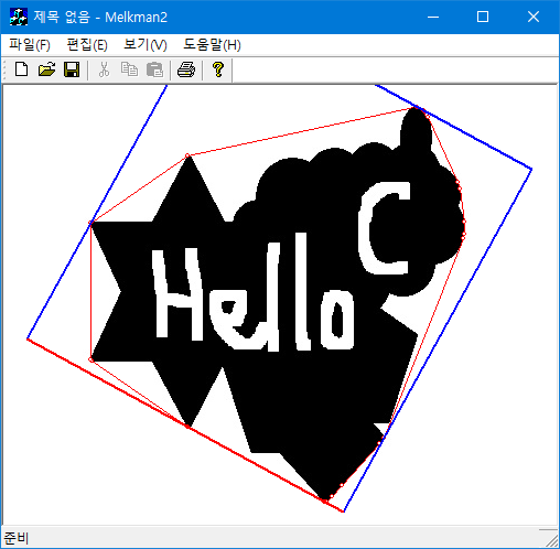
주어진 점집합을 포함하는 최소 면적의 rectangle을 찾는 문제는 점집합의 convex hull을 포함하는 rectangle을 찾는 문제와 같다. convex hull의 한 변을 공유하면서 전체를 포함하는 rectangle 중 최소 면적인 것을 찾으면 된다. Rotating Caliper를 쓰면 O(n) step이 요구된다.

// 방향이 dir이고 A점을 통과하는 직선과 방향이 dir에 수직이고 B점을 통과하는 직선의 교점을 반환;
CPoint LineIntersect(CPoint A, CPoint dir, CPoint B);
//
#define DOT(A,B) ((A).x*(B).x + (A).y*(B).y))
void BoundingRect(std::vector<CPoint>& hull, CPoint vtx[4]) {//non-optimal.
    if (hull.size() < 3) return;
    double minArea = DBL_MAX;
    int bIndex = 0, tIndex = 0, lIndex = 0, rIndex = 0;
    for (int j = 0, i = hull.size() - 1; j < hull.size(); i = j++) {
        CPoint &A = hull[i], &B = hull[j];
        CPoint BA = B - A;  // convex hull의 한 기준변;
        CPoint BAnormal = CPoint(-BA.y, BA.x); //(B-A)에 반시계방향으로 수직인 벡터;
        double BAsq = DOT(BA, BA);
        //기준변과 대척점(antipodal point)을 찾는다: BAnormal방향으로 가장 멀리 떨어진 점
        int id = FindAntipodal(BAnormal, hull) ;
        CPoint QA = hull[id] - hull[i];
        //기준변과 대척점을 통과하는 직선과의 사이거리;
        double D1 = fabs(double(DOT(BAnormal, QA))) / sqrt(BAsq);
        //left_side_end_point;//기준변 반대방향으로 가장 멀리 떨어진 꼭지점;
        int id1 = FindAntipodal(-BA, hull);
        //right_side_end_point;//기준변 방향으로 가장 멀리 떨어진 꼭지점;
        int id2 = FindAntipodal(BA, hull);

        ///가장 왼쪽과 가장 오른쪽 꼭지점을 연결하는 선분
        CPoint H = hull[id1] - hull[id2];  
        //기준변 방향으로 정사영하면 두 평행선 사이거리를 줌;
        double D2 = fabs(double(DOT(BA,H))) / sqrt(BAsq);
        double area = D1 * D2; 
        if (area < minArea) {
            minArea = area;
            bIndex = i ;  tIndex = id;
            lIndex = id1; rIndex = id2;
        }
    }
    //directional vector for base_edge;
    CPoint dir = hull[(bIndex + 1) % hull.size()] - hull[bIndex] ; 
    vtx[0] = LineIntersect(hull[bIndex], dir, hull[lIndex]);
    vtx[1] = LineIntersect(hull[tIndex], dir, hull[lIndex]);
    vtx[2] = LineIntersect(hull[tIndex], dir, hull[rIndex]);
    vtx[3] = LineIntersect(hull[bIndex], dir, hull[rIndex]);
}

각 전경 픽셀에 대해서 모든 배경 픽셀까지 거리를 구한 다음 최솟값을 할당하면 된다. 픽셀 수가 n = w * h 개면 time complexity는 O(n^2)이다 (이미지 폭이나 높이의 4승이므로 연산량이 상당하다.) linear time Euclidean distance transform은 kipl.tistory.com/268.

ListPlot3D[ Reverse@ImageData[pic], PlotRange -> Full]

int brute_force_edt(double *img, int w, int h) {
    int *list = new int [w * h];
    int fg_cnt = 0;
    int bg_ptr = w * h;               //배경 픽셀 위치는 끝에서 역으로 채움;
    //전경과 배경 픽셀 위치를 분리;
    for (int i = w * h; i-->0;)
        if (img[i]) list[fg_cnt++] = i;  // foreground;
        else        list[--bg_ptr] = i;  // background;

    for (int i = 0; i < fg_cnt; ++i) {     // 전경 픽셀;
        int xi = list[i] % w, yi = list[i] / w;
        double d2min = DBL_MAX;
        for (int j = w * h; j--> fg_cnt;) { // 배경 픽셀까지 거리를 계산해서 최소값을 할당;
                                          // 배경이 list에 역순으로 저장됨으로 역방향 서치;
            int xj = list[j] % w, yj = list[j] / w;
            double dx  = xi - xj, dy = yi - yj;  //
            double dst = dx * dx + dy * dy;
            if (dst == 1) {
            	d2min = 1; break;
            }
            if (d2min > dst) d2min = dst;
        }
        img[list[i]] = d2min;
    }
    delete [] list;
    return fg_cnt;
}

평균이 $\lambda$인 Poisson 분포를 가지는 random number를 만드는 레시피는 [0,1]에서 추출된 균일한 random number 수열이 $u_1, u_2, u_3,...$로 주어질 때, $u_1  u_2 u_3....u_{k+1}\le  e^{-\lambda}$을 처음 만족하는 $k$를 찾으면 됨이 Knuth에 의해서 알려졌다.

int PoissonValue(double lambda) { // lambda = mean value
    double L = exp(-lambda);
    int k = 0;
    double p = 1;
    do {
        k++;
        // generate uniform random number u in [0,1] and let p ← p × u.
        p *= double(rand()) / RAND_MAX;
    } while (p > L);
    return (k - 1);
}

이미지에서 각각의 픽셀 값은 영상신호를 받아들이는 ccd 센서에서 노이즈가 포함된 전기신호(광자 수)의 평균값이 구현된 것으로 볼 수 있다. 따라서 영상에 Poisson 노이즈를 추가하는 과정은 역으로 주어진 픽셀 값을 평균으로 가지는 Poisson 분포의 램덤 변수를 픽셀값으로 대체하면 된다.(물론 이미지에 무관하게 노이즈를 추가할 수도 있다. 예를 들면 모든 픽셀에 대해서 같은 평균값을 갖는 포아송 노이즈를 주는 경우다)

void AddPoissonNoise(CRaster& raster, CRaster& noised) {
    if (raster.IsEmpty() || raster.GetBPP() != 8) return;
    CSize sz = raster.GetSize();
    noised = raster;
    srand(unsigned(time(0)));
    for (int y = 0; y < sz.cy; y++) {
        BYTE *p = (BYTE *)raster.GetLinePtr(y);
        BYTE *q = (BYTE *)noised.GetLinePtr(y);
        for (int x = 0; x < sz.cx; x++) {
            int a = PoissonValue(*p++);
            *q++ = a > 0xFF ? 0xFF: a;
        }
    }
}

아래 예제는 cos(t)로 표현되는 신호에 Poisson noise를 주는 경우를 보여준다. Poisson noise 함수는 신호값을 평균으로 주는 event의 횟수를 찾아주므로 음수의 신호는 바로 다룰 수 없다. 따라서 원신호에 +1 만큼 더해 준 신호를 기준으로 한다. 그런데 cos(t) + 1의 범위가 [0,2]이므로 이산분포인 Poisson 분포를 적용하기 위해서는 적당한 스케일링이 필요하다. 예를 들면 cos(t) + 1이 신호의 절대값을 측정한 것이 아닌 상대적인 세기를 나타내고, 실제 신호의 최대값은 50으로 주어졌다면 Poisson noise을 만들 때 평균값이 주어진 신호 함수의 50배인 경우에 해당하는 값을 입력으로 넣은 후 출력값을 다시 50으로 나누어주면 된다.

void PoissonNoiseEx1D() {
    FILE *fp = fopen("poisson.txt", "w");
    for (double t = 0; t < 10; t += 0.01) {
        double y = cos(t) + 1.;
        fprintf(fp, "%f %f %f\n", t, y, (double)PoissonValue(y * 50) / 50.);
    }
    fclose(fp);
}

Poisson 잡음은 random noise처럼 단순히 더해지는 잡음과 달리 신호값이 클 때 잡음도 더 커짐을 알 수 있다. 그러나 SNR은 신호값이 클수록 더 좋아진다.

$$\text{distance measure}:~\text{Manhattan distance}=|x_2 - x_1 | + |y_2 - y_1|$$

Grassfire 알고리즘을 써서 최단경로를 찾는 문제는 DFS로도 구현할 수 있으나 비효율적이고(왜 그런지는 쉽게 알 수 있다) BFS로 구현하는 것이 더 적합하다. 

void grassfire(CPoint q, int **map, int w, int h, int **dist) {
    // left-top-right-bottom;
    const int dx[] = {-1,  0, 1, 0};
    const int dy[] = { 0, -1, 0, 1};
    for (int y = 0; y < h; y++) 
        for (int x = 0; x < w; x++) 
            dist[y][x] = INF;  //unvisited cells;

    std::queue<CPoint> Q;
    dist[q.y][q.x] = 0;     //start( or end) position: distance = 0;
    Q.push(q);
    while (!Q.empty()) {
        CPoint p = Q.front(); Q.pop();
        int distance = dist[p.y][p.x];
        // 4-way search;
        for (int i = 0; i < 4; i++) {
            CPoint q = CPoint(p.x + dx[i], p.y + dy[i]);
            if (q.x < 0|| q.y < 0|| q.x >= w|| q.y >= h) continue;
            if (map[q.y][q.x] == 0 && dist[q.y][q.x] == INF) {
                dist[q.y][q.x] = distance + 1;
                Q.push(q);
            }
        }
    }
};
// back tracking;
CPoint back_track(CPoint p, int **dist, int w, in h) {
    // left-top-right-bottom;
    const int dx[] = {-1,  0, 1, 0};
    const int dy[] = { 0, -1, 0, 1};
    int depth = dist[p.y][p.x]; 
    if (--depth < 0) return p;
    for (int i = 0; i < 4; i++) {
        CPoint q = CPoint(p.x + dx[i], p.y + dy[i]);
        if (q.x < 0 || q.y < 0 || q.x >= w || q.y >= h) continue; // out of ROI;
        else if (dist[q.y][q.x] == depth)
            return q;
    }
    return p; // never hit;
}

평면 위에서 주어진 점집합을 포함하는 가장 작은 원을 찾는 문제는 가장 단순하게는 임의의 두 점이 지름이 되는 원과 임의의 세 점이 만드는 외접원을 모두 조사하여 찾으면 된다. 따라서 O(n^4)의 복잡도를 가질 것이다. 그러나 이 문제는 점집합의 갯수에 비례하는 시간 복잡도(O(n))를 가지는 알고리즘이 알려져 있고, 여기서는 재귀적 방법을 이용한  Welzl's algorithm을 구현한다.

int MinEncCir ( CfPt *P, int n, CfPt* boundary, int b, CfPt& center, double& rad ) {
    // exiting cases
    if ( b == 3 ) CalcCircle3 ( boundary, center, rad ); // a circle passing 3 points;
    else if ( ( n == 1 ) && ( b == 0 ) ) {
        rad = 0; b = 1;
        center = boundary[0] = P[0];
    } 
    else if ( ( n == 2 ) && ( b == 0 ) ) {
        boundary[0] = P[0]; boundary[1] = P[1]; b = 2;
        CalcCircle2 (boundary, center, rad );  // a circle with diagonal consisting of 2 points;
    }
    else if ( ( n == 0 ) && ( b == 2 ) ) {
        CalcCircle2 ( boundary, center, rad );
    }
    else if ( ( n == 1 ) && ( b == 1 ) ) {
        boundary[1] = P[0]; b = 2;
        CalcCircle2 ( boundary, center, rad );
    }
    else {// general case; ( b < 3 ) && ( n + b > 2 )
        // choose a random pivot;
        int k = rand() % n;
        if ( k != 0 ) SWAP( P[0], P[k] );
        int b1 = MinEncCir ( &P[1], n - 1, boundary, b, center, rad );
        if (!InCircle(P[0], center, rad) ) {
            // Now, P[0] belongs to the boundary.
            boundary[b++] = P[0];
            return MinEncCir ( &P[1], n - 1, boundary, b, center, rad );
        } else return b1;
    }
    return b;
}