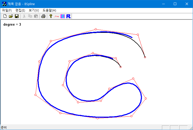
$m$개의 control point $\{\mathbf{Q}_i\}$가 주어지면  $p$차의 B-Spline curve는 basis 함수를 $N_{i, p}(t)$을 써서

$$ \mathbf{B}(t) = \sum_{i=0}^{m-1} N_{i, p}(t) \mathbf{Q}_i $$

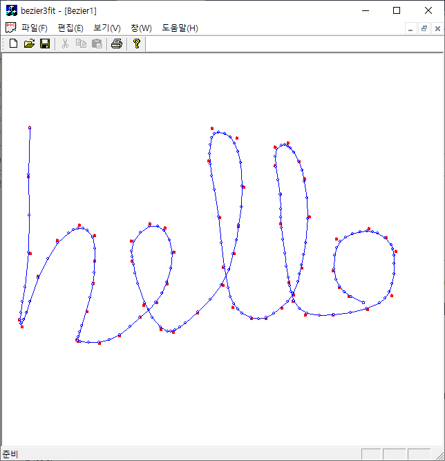
로 표현할 수 있다. 이를 이용해서 일정한 순서로 샘플링된 평면상의 $N$개의 입력점 $\{ \mathbf{P}_i \}$을 찾아보자. B-spline 곡선을 이용하면 이 문제는 control 점을 찾는 문제가 된다. 곡선이 입력점을 잘 표현하기 위해서는 곡선과 입력점과의 차이를 최소로 하는 control 점을 찾아야 한다:

$$    \mathbf{ Q}^* = \text{argmin}(L), \quad\quad L:= \sum_{k = 0}^{N-1} | \mathbf{B}(t_k) - \mathbf{P}_k|^2 $$

여기서 $\{ t_k| k=0,1,...,N-1\}$는 입력점이 얻어지는 sample time으로 $0= t_0\le t_1\le...\le t_{N-1}= 1$로 rescale 할 수 있다. 

행렬을 이용해서 식을 좀 더 간결하게 표현할 수 있다. 

$$L = \sum_{k = 0}^{N-1} | \mathbf{B}(t_k) - \mathbf{P}_k|^2 = \sum_{k = 0}^{N-1} \left| \sum_{i=0}^{m-1} N_{i, p}(t_k) \mathbf{Q}_i -  \mathbf{P}_k \right|^2 = \sum_{k = 0}^{N-1} \left| \sum_{i=0}^{m-1} A_{ki} \mathbf{Q}_i - \mathbf{P}_k \right|^2, \\ \quad A_{ki} = N_{i, p}(t_k) $$

로 쓸 수 있으므로, $\hat {Q}= (\mathbf{Q}_0, \mathbf{Q}_1,..., \mathbf{Q}_{m-1})^t$, $\hat {P} = (\mathbf{P}_0, \mathbf{P}_1,..., \mathbf{P}_{N-1})^t$인 벡터, 그리고 $ \hat {A} = (A_{ki})$인 행렬로 보면

$$ L= \left| \hat{A} \cdot \hat {Q} - \hat {P} \right|^2 =  (\hat{Q}^t \cdot \hat {A}^t -\hat{P}^t ) \cdot (\hat{A}\cdot \hat{Q} - \hat{P}).$$

위 식의 값을 최소로 하는 최소자승해는 $\hat {Q}^t$에 대한 미분 값이 0인 벡터를 찾으면 된다; $$ \frac {\partial L}{\partial \hat {Q}^t } = \hat {A}^t \cdot \hat {A} \cdot \hat {Q} - \hat {A}^{t} \cdot \hat {P} = 0.$$ 이 행렬 방정식의 해는

$$ \hat {Q}^* = ( \hat {A} ^t \cdot \hat {A})^{-1} \cdot ( \hat {A}^t \cdot \hat {P})$$ 로 표현된다. $\hat {A} ^t \cdot \hat {A}$가 (banded) real symmetric ($m\times m$) 행렬이므로 Cholesky decomposion을 사용하면 쉽게 해를 구할 수 있다. $\hat{A}$가 banded matrix 형태를 가지는 이유는 basis가 local support에서만 0이 아닌 값을 취하기 때문이다. 

open b-spline(cubic)

int BSplineFit_LS(std::vector<CPoint>& data,
                  int degree,             // cubic(3); 
                  int nc,                 // num of control points;
                  std::vector<double>& X,
                  std::vector<double>& Y) // estimated control points;
{
    // open b-spline;
    std::vector<double> knot((nc - 1) + degree + 2);
    for (int i = 0; i <= nc + degree; i++) knot[i] = i;
    
    std::vector<double> t(data.size());       // parameter;
    double scale = (knot[nc] - knot[degree]) / (data.size()-1);
    for (int i = data.size(); i-->0;) 
        t[i] = knot[degree] + scale * i;

    std::vector<double> A(ndata * nc);
    for (int i = data.size(); i-->0;)
        for (int j = 0; j < nc; j++)
            A[i * nc + j] = Basis(j, degree, &knot[0], t[i]); //A(i,j)=N_j(t_i)

    // S = A^t * A; real-symmetric matrix;
    std::vector<double> Sx(nc * nc);
    std::vector<double> Sy(nc * nc);
    for (int i = 0; i < nc; i++) {
        for (int j = 0; j < nc; j++) {
            double s = 0;
            for (int k = data.size(); k-->0;)
                s += A[k * nc + i] * A[k * nc + j];
            Sx[i * nc + j] = s;
        }
    }
    //copy;
    for (int i = nc*nc; i-->0;) Sy[i] = Sx[i];
    // X = A^t * P.x;  Y = A^t * P.y
    for (int i = 0; i < nc; i++) {
        double sx = 0, sy = 0;
        for (int k = data.size(); k-->0;) {
            sx += A[k * nc + i] * data[k].x;
            sy += A[k * nc + i] * data[k].y;
        };
        X[i] = sx; Y[i] = sy;
    };
    // solve real symmetric linear system; S * x = X, S * y = Y;
    // solvps(S, X) destories the inputs;
    // ccmath-2.2.1 version;
    int res1 = solvps(&Sx[0], &X[0], nc);
    int res2 = solvps(&Sy[0], &Y[0], nc);
    return res1 == 0 && res2 == 0;
};

**네이버 블로그 이전;

 
728x90

'Computational Geometry' 카테고리의 다른 글

Approximate Distance Between Ellipse and Point  (0) 2024.03.08
Distance from a Point to an Ellipse  (0) 2024.03.06
Closest Pair of Points  (0) 2021.04.27
DDA Algorithm  (0) 2021.04.25
B-Spline  (0) 2021.04.25
Posted by helloktk
,

Brute-force : O(n^2),

Optimal: O(n log(n))

참고: people.csail.mit.edu/indyk/6.838-old/handouts/lec17.pdf

참고: arxiv.org/pdf/1911.01973.pdf

//  points should be sorted in order of increasing x-component.
//
#define DIST2(p, q) ((p).x-(q).x)*((p).x-(q).x) + ((p).y-(q).y)*((p).y-(q).y)
// 수정: index range -> [left, right]; ClosestPair(points, 0, points.size()-1, closest);
int ClosestPair(std::vector<CPoint>& points, int left, int right, int closest[2]) {
    if (right - left >= 3) {
        int lpair[2], rpair[2], min_dist2;
        int mid = left + (right - left) / 2;                    // half index;
        int ldist = ClosestPair(points, left, mid, lpair);     // left side;
        int rdist = ClosestPair(points, mid+1, right, rpair); // right side;
        if (ldist < rdist) {
            closest[0] = lpair[0]; closest[1] = lpair[1];
            min_dist2 = ldist;
        } else {
            closest[0] = rpair[0]; closest[1] = rpair[1];
            min_dist2 = rdist;
        }
        // find points which lies near center strip(2d-strip);
        // Note our distance is the squar of actual distance;
        int width = int(sqrt(double(min_dist2))+ .5);
        int ll = left;
        while (points[ll].x < (points[mid].x - width - 1)) ll++;
        int rr = idx2;
        while (points[rr].x > (points[mid + 1].x + width + 1)) rr--;
        for (int i = ll; i < rr; i++) {
            for (int j = i + 1; j <= rr; j++) {
                int dist2 = DIST2(points[i], points[j]);
                if (min_dist2 > dist2) {
                    min_dist2 = dist2;
                    closest[0] = i; closest[1] = j;
                }
            }
        }
        return min_dist2;
    } 
    else if (right == left + 2) {
        return ClosestPair3(points, left, closest);
    }
    else if (right == left + 1) {
        closest[0] = left; closest[1] = right;
        return DIST2(points[left], points[right]);
    }
    else return INT_MAX;
};
 
 
728x90

'Computational Geometry' 카테고리의 다른 글

Distance from a Point to an Ellipse  (0) 2024.03.06
Data Fitting with B-Spline Curves  (0) 2021.04.30
DDA Algorithm  (0) 2021.04.25
B-Spline  (0) 2021.04.25
Bezier Smoothing  (0) 2021.04.23
Posted by helloktk
,

Fixed-point version: 선분 길이가 4096 픽셀 정도까지는 1-pixel 이내의 오차로 그려진다.

void DDALine(CPoint A, CPoint B) {
    const int mulfac = 4096; // 2^12 = 4096;
    int dx = B.x - A.x;
    int dy = B.y - A.y;
    int adx = dx < 0 ? -dx : dx;
    int ady = dy < 0 ? -dy : dy;
    int steps = adx < ady ? ady : adx;
    if (steps == 0) SetPixel(A.x, A.y); //single point;
    else {
        int curX = A.x * mulfac;      
        int curY = A.y * mulfac;
        dx = (dx * mulfac) / steps;
        dy = (dy * mulfac) / steps;
        while (steps-- >= 0) {
            SetPixel(curX / mulfac, curY / mulfac);
            curX += dx;
            curY += dy;
        }
    }
}
728x90

'Computational Geometry' 카테고리의 다른 글

Data Fitting with B-Spline Curves  (0) 2021.04.30
Closest Pair of Points  (0) 2021.04.27
B-Spline  (0) 2021.04.25
Bezier Smoothing  (0) 2021.04.23
Flatness of Cubic Bezier Curve  (0) 2021.04.23
Posted by helloktk
,

B-Spline

Computational Geometry 2021. 4. 25. 09:43

$$ \mathbf{C}(u) = \sum_{i=0}^{n} N_{i,p} (u) \mathbf{P}_i$$

where $N_{i, p}(u)$'s are B-spline basis functions of degree $p$, $n+1$ control points $\{\mathbf{P}_i\}$, and a knot vector $\mathbf{U}=(u_0, u_1, ..., u_m)$. Note, $m=n + p + 1$.

B-spline의 basis 함수 $N_{i, p}(t)$는 유한한 구간에서만 0이 아닌 값을 갖는(local support) 함수로 다음과 같은  recursion relation을 가진다:

\begin{align} N_{i,0}(t) &= \left\{ \begin{matrix} 1 & \mathrm{if} \quad u_i \leq x \lt u_{i+1} \\ 0 & \mathrm{otherwise} \end{matrix} \right. \quad \quad (0 \le i \le n+p), \\ N_{i,p}(t) &= \frac{t - u_i}{u_{i+p} - u_i} N_{i,p-1}(t) + \frac{u_{i+p+1} - t}{u_{i+p+1} - u_{i+1}} N_{i+1,p-1}(t).\end{align}

$N_{i,p}(t)$의 local support는 $[u_i, u_{i+p+1}]$로 주어진다.

일반적으로 knot vector가 특별한 구조를 가지지 않으면 B-spline곡선은 Bezier 곡선의 경우와 달리 처음과 끝 control 점을 통과하지 않는다(open B-spline). 처음과 끝점을 통과하도록 만들기 위해서는 knot 벡터의 시작 $(p+1)$개 성분이 같은 값을 갖고, 마지막 $(p+1)$개 성분도 같은 값을 갖도록 조정하면 된다(clamped B-spline):

$$clamped: u[0]=u[1]=...=u[p],...,u[n+1]=...=u[n+p]=u[n+p+1]$$

knot는 균일할 필요는 없지만, 균일한 경우는 보통

$$ u_i = \left\{ \begin{array} {rcl} 0 & , & 0 \le i \le p, \\ \frac{i-p}{n+1-p}&, & p+1\le i \le n \\ 1&,& n+1\le i \le n+p+1\end{array}\right.$$

로 선택한다. 

ref: ae.sharif.edu/~aerocad/curve%20modelling-B_Spline.pdf

clamped(black), open(blue)

// Note, p = degree;
void BSpline(int p, std::vector<CPoint>& control, int resolution, CDC *pDC) {
    int n = control.size() - 1;  ASSERT(n > 0);
    std::vector<double> u(n + p + 2);                // knot vector;
    calculateKnots(&u[0], n, p);                     // uniform knot;
    double delta = (u[n + p + 1] - u[0]) / (resolution - 1);  // parameter increment;
    CPoint Q;
    for (double t = u[0] ; t <= u[n+p+1]; t += delta) {
        calculatePoint(&u[0], n, p, t, &control[0], &Q);
        if (i == 0) pDC->MoveTo(Q);
        pDC->LineTo(Q);
    }
    pDC->LineTo(control[n]);
}
// de Boor Cox's algorithm;
double Blend(int i, int p, double *u, double t) {  
    if (p == 0) { // termination condition of recursion;
        if ((u[i] <= t) && (t < u[i+1]))        return 1;
        else                                    return 0;
    }
    else {
        double coef1, coef2;
        if (u[i+p] == u[i]) {
            if (t == u[i])  coef1 = 1;
            else            coef1 = 0;
        } 
        else                coef1 = (t - u[i]) / (u[i+p] - u[i]); 
        
        if (u[i+p+1] == u[i+1]) {
           if (t == u[i+1]) coef2 = 1;
           else             coef2 = 0;
        } 
        else                coef2 = (u[i+p+1] - t) / (u[i+p+1] - u[i+1]);
        return coef1 * Blend(i, p-1, u, t) + coef2 * Blend(i+1, p-1, u, t);
    }
}
// clamped b-spline knot vector; uniform example;
// u[0]=u[1]= ... =u[p],.....,u=[n+p-2]=u[n+p-1]=u[n+p]=u[n+p+1]
void calculateKnots(double *u, int n, int p) {
    int j = 0; 
    while (j <= p)     u[j++] = 0;                 // multiplicity = p+1;
    while (j <= n)     u[j++] = j - p;             // m = n+p+1;
    while (j <= n+p+1) u[j++] = n - p + 1;         // multiplicity = p+1;
}
void calculatePoint(double *u, int n, int p, double t, CPoint *control, CPoint *output) {
    double x = 0, y = 0;
    for (int i = 0; i <= n; i++) {
        double b = Blend(i, p, u, t);
        x += control[i].x * b;
        y += control[i].y * b;
    }
    output->x = int(x + 0.5);
    output->y = int(y + 0.5);
}
728x90

'Computational Geometry' 카테고리의 다른 글

Closest Pair of Points  (0) 2021.04.27
DDA Algorithm  (0) 2021.04.25
Bezier Smoothing  (0) 2021.04.23
Flatness of Cubic Bezier Curve  (0) 2021.04.23
Convexity of Bezier Curve  (0) 2021.04.22
Posted by helloktk
,

입력점들을 부드럽게 연결하는 베지어 곡선을 찾아보자. 입력점 사이 구간을 3차 베지어 곡선으로 표현하려면  4개의 컨트롤점이 필요한데, 최소자승법을 이용하지 않고 순차적인 3 입력점 $P_0, P_1, P_2$이 주어질 때 이를 이용해서 컨트롤 점을 구성한다.(따라서 베지어 곡선은 시작과 끝이 아닌 입력점을 일반적으로 통과하지 않는다)  $$C_0 = (P_0+P_1)/2,~~C_1 = (P_0 +5 P_1)/6,~~C_2 = (5P_1+  P_2)/6,~~C_3=(P_1+P_2)/2$$ 컨트롤점으로 하는 베지어 곡선은  $[P_0, P_1, P_2]$의 일부분을 표현한다. 이 과정은 다음 한 입력점을 포함시켜서 다시 반복을 하는데 이 떄  이전 베이어 곡선의 마지막 컨트롤점($C_2$)이 새로이 만들어지는 베지어 곡선의 시작점($C_0^\text{new}$)이 되므로 두 베지어 곡선은 부드럽게 연결이 된다. 입력점의 시작과 끝점은 베이어 곡선이 통과하도록 컨트롤점에 포함되게 설계한다.

$$\text{front}:~ C_0=P_0, ~~C_1 = (P_0+2P_1)/3$$

$$\text{back}:~C_2=(2P_1+P_2)/3, ~~C_3=P_3$$

그리고 주어진 베지어 곡선의 분할은 균일한 간격으로 하지 않고, 각각의 구간에서 베지어 곡선이 충분히 평탄하도록 분할해서 저장한다.

// test flatness of a bezier curve with control points {p1, c1, c2, p2};
bool FlatBezier(const double eps, 
                const CfPt& p1, const CfPt& c1, const CfPt& c2, const CfPt& p2) {
    CfPt U = c1 - (p1 * 2 + p2) / 3;
    CfPt V = c2 - (p1 + p2 * 2) / 3;
    double normU = hypot(U.x, U.y);
    double normV = hypot(V.x, V.y);
    return (3. * max(normU, normV) / 4.) <= eps;
}
// subdivision stage; De Casteljau's algorithm
void GetBezierPoints(const double eps, 
                     const CfPt &p1, const CfPt &c1, const CfPt &c2, const CfPt &p2,
                     std::vector<CfPt>& smoothed) {
    if (!FlatBezier(eps, p1, c1, c2, p2)) {
        // Subdivide the curve at t = 0.5
        // left;
        CfPt mid_segm = (p1  + c1 * 3 + c2 * 3 + p2) / 8.0; // = B(1/2);
        CfPt new_c1   = (p1 + c1) / 2.0;
        CfPt new_c2   = (p1 + c1 * 2 + c2) / 4.0;   // ((p1+c1)/2+(p1+c2)/2)/2
        GetBezierPoints(eps, p1, new_c1, new_c2, mid_segm, smoothed);
        // right;
        new_c1  = (c1 + c2 * 2 + p2) / 4.0;
        new_c2  = (c2 + p2) / 2.0;
        GetBezierPoints(eps, mid_segm, new_c1, new_c2, p2, smoothed);
    } 
    else smoothed.push_back(p2); // flat enough;
        
}
// linear interpolation between a and b;
// a와 b 사이를  (1-t): t로 내분;
CfPt lerp(const double t, const CfPt &a, const CfPt &b) {
    return a * (1 - t) + b * t;
}
void SmoothPathWithBezier(std::vector<CfPt>& points, std::vector<CfPt>& smoothed) {
    if (points.size() < 3) return ;
    CfPt cntl[4];
    CfPt *pts = &points[0];   // iterator;
    const int N = points.size();   
    smoothed.clear();
    smoothed.push_back(pts[0]);    
    for (int i = 2; i < N; i++, pts++) {
        if (i == 2) {
            cntl[0] = pts[0];
            cntl[1] = lerp(2./ 3, pts[0], pts[1]);
        } else {
            //0번 control-pts= (0-1)의 중간점;
            //1번 control-pts= (0-1)의 5:1 내분점; 
            cntl[0] = lerp(1./ 2, pts[0], pts[1]);
            cntl[1] = lerp(5./ 6, pts[0], pts[1]);
        }
        if (i == N-1) {
            //1:2 내분점;
            cntl[2] = lerp(1./ 3, pts[1], pts[2]);
            cntl[3] = pts[2];
        } else {
            //2번 control-pts;(1-2)의 1:5 내분점;
            //3번 control-pts;(1-2)의 중간점;
            cntl[2] = lerp(1./ 6, pts[1], pts[2]);
            cntl[3] = lerp(1./ 2, pts[1], pts[2]);
        }
        //입력 중에 처음 두개가 같거나, 다음 두개가 같으면 마지막이 충분히 smooth하므로 
        // 마직막 control pt만 베지어 곡선에 삽입;
        if ((pts[0] == pts[1]) || (pts[1] == pts[2])) 
            smoothed.push_back(cntl[3]);
        else {
            double tolerance = 1.; // 1-pixel;
            GetBezierPoints(tolerance, cntl[0], cntl[1], cntl[2], cntl[3], smoothed);
        }
    }
}
728x90

'Computational Geometry' 카테고리의 다른 글

DDA Algorithm  (0) 2021.04.25
B-Spline  (0) 2021.04.25
Flatness of Cubic Bezier Curve  (0) 2021.04.23
Convexity of Bezier Curve  (0) 2021.04.22
De Casteljau's Algorithm  (0) 2021.04.22
Posted by helloktk
,