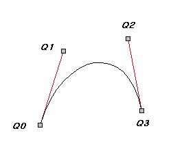
cubic Bezier 곡선은 네 개의 컨트롤 점 ($\bf {P}_0, P_1, P_2, P_3$)이용해서 표현한다:
$$\mathbf {B}(t) = (1-t)^3 \mathbf {P}_0 + 3(1-t)^2 t \mathbf {P}_1 + 3 (1-t) t^2 {\bf B}_2 + t^3 \mathbf {P}_3. \quad 0 \le t \le 1 \\{\bf B}(0) ={\bf P}_0 , ~~ {\bf B}(1) = {\bf P}_3$$
만약 곡선이 충분히 평탄하다면 굳이 삼차 다항식을 계수로 가지는 Bezier 곡선으로 표현할 필요가 없이$\mathbf {P}_0$와 ${\bf P}_3$을 잇는 직선으로 근사하는 것이 여러모로 유리할 것이다. 그러면 Bezier 곡선의 평탄성을 어떻게 예측할 것인가? 이는 cubic Bezier 곡선 ${\bf B}(t)$와 시작점과 끝점을 연결하는 직선 $\mathbf {L}(t)= (1-t) \mathbf {P}_0 + t \mathbf {P}_3$와의 차이를 비교하므로 판단할 수 있다.
직선도 cubic Bezier 곡선 표현으로 할 수 있다. 시작점이 $\mathbf {P}_0$이고 끝점이 $\mathbf {P}_3$일 때 이 둘 사이를 3 등분하는 두 내분점 $(2\mathbf {P}_0 + \mathbf{P}_3)/3$, $( \mathbf {P}_0 + 2\mathbf {P}_3)/3$을 control point에 포함시키면,
$$\mathbf {L}(t)= (1-t)^3 \mathbf {P}_0 + (1-t)^2 t (2 \mathbf {P}_0 +\mathbf {P}_3)+ (1-t) t^2 (\mathbf {P}_0 + 2 \mathbf {P}_3)+ t^3 \mathbf {P}_3$$
처럼 쓸 수 있다. Bezier 곡선과 직선의 차이를 구하면
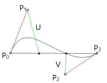
\begin{align} \Delta (t) &= |\mathbf {B}(t) - \mathbf {L}(t)| \\ &= |(1-t)^2 t (3\mathbf {P}_1 -2 \mathbf {P}_0 -\mathbf{P}_3) + (1-t) t^2(3 \mathbf {P}_2 - \mathbf {P}_0 - 2 \mathbf {P}_3)| \\ &= 3 (1-t) t |(1-t) \mathbf {U} + t \mathbf {V}|, \\ \\ &\quad \mathbf {U}=\mathbf {P}_1 - \frac{1}{3}(2 \mathbf {P}_0 + \mathbf {P}_3), \quad \mathbf {V}=\mathbf {P}_2 - \frac{1}{3} (\mathbf {P}_0 + 2 \mathbf {P}_3) \end{align}
그런데
$$ \text {max} \{3(1 - t) t \} = \frac {3}{4}, \quad 0\le t \le 1, \\ \text {max}\{ |(1-t) \mathbf {U} + t \mathbf {V}| \} =\text {max}\{ |\mathbf{U}| , |\mathbf {V}|\} $$
이므로 아래와 같은 벗어난 거리의 상한 값을 얻을 수 있다:
$$ \Delta (t) \le \frac {3}{4} \text{max} \{ |\mathbf {U} | , |\mathbf {V}| \}$$
이 상한값이 주어진 임계값보다 작으면 3차 Bezier 곡선은 두 끝점을 잇는 직선으로 근사할 수 있다. 좀 더 기하학적으로 표현하면
$$|\mathbf{U}| = \mathbf{P}_1\text{에서 왼쪽 3등분 내분점까지 거리}$$
$$|\mathbf {V}|= \mathbf {P}_2 \text{에서 오른쪽 3등분 내분점까지 거리}$$
이므로,
$$ \Delta(t) \le \frac {3}{4}\times( \text{control point와 3등분 내분점 간의 거리의 최댓값}).$$
'Computational Geometry' 카테고리의 다른 글
| B-Spline (0) | 2021.04.25 |
|---|---|
| Bezier Smoothing (0) | 2021.04.23 |
| Convexity of Bezier Curve (0) | 2021.04.22 |
| De Casteljau's Algorithm (0) | 2021.04.22 |
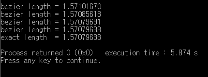
| Arc Length of Bezier Curves (0) | 2021.04.21 |