Geometry & Recognition

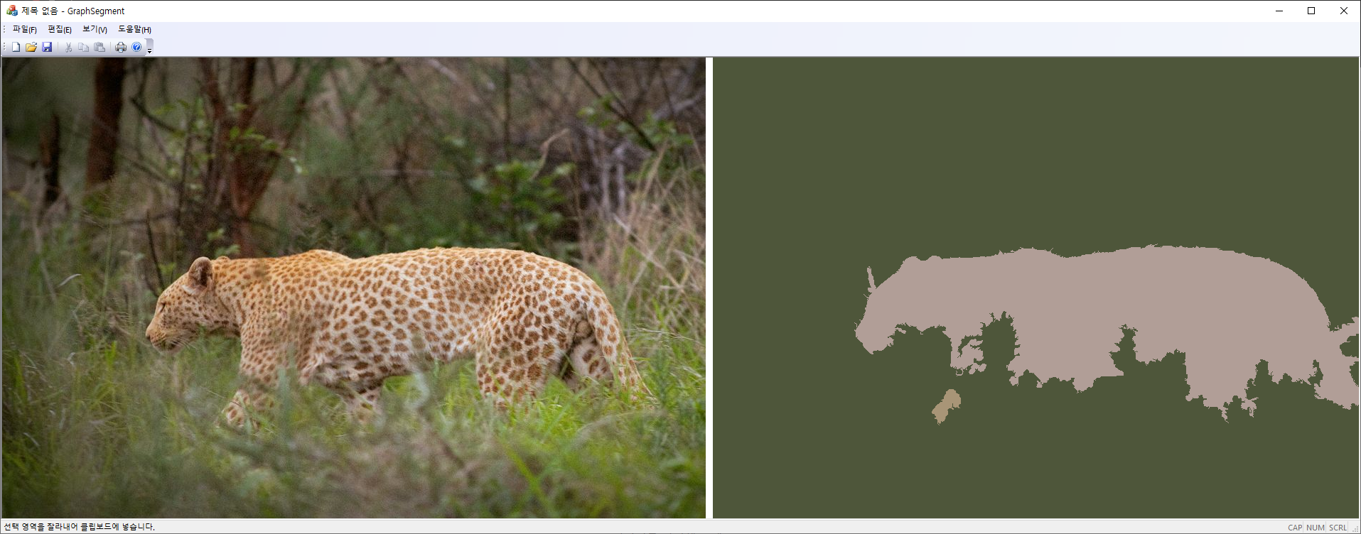
comb 함수: 일정한  간격($T$)으로 주어진 message를 샘플링하는 함수.

$$\text{comb}_T(t) := \sum_{n=-\infty}^{\infty} \delta (t- nT)$$

주기가 $T$인 함수다: 

$$ \text{comb}_T(t) = \text{comb}_T(t+T)$$

따라서 Fouries series 전개가 가능하다.

$$\text{comb}_T(t) = \sum_{n=-\infty}^{ \infty}   c_n e^{i 2\pi n t /T}$$

계수 $c_n$은?

\begin{align} c_n :=&\frac{1}{T} \int_{-T/2}^{T/2} \text{comb}_T(t) e^{-i 2\pi n t /T}dt \\ =&  \frac{1}{T}\int_{-T/2}^{T/2} \delta (t) e^{ -i 2\pi n t/T} dt  \\ =&\frac{1}{T} e^{-i 2\pi n (0) /T } = \frac{1}{T}.\end{align}

따라서, $\text{comb}_T(t)$의 Fourier series 전개는 

$$\text{comb}_T(t) = \frac{1}{T} \sum_{n = -\infty}^{\infty} e^{i2\pi  n t/T}.$$

frequency domain에서 delta 함수의 역 Fourier transform은 정의에 의해서

$$ {\cal F}^{-1} [\delta (f-f_0)] = \int \delta (f-f_0) e^{i 2\pi t f }df = e^{i 2\pi t f_0}$$

그럼 $\text{comb}_T(t)$의 Fourier transform은 어떻게 표현되는가?

\begin{align} {\cal F}[\text{comb}_T(t)]=& \frac{1}{T} \sum {\cal F}[ e^{i2\pi n t/T}] \\  =& \frac{1}{T} \sum {\cal F}[ {\cal F}^{-1} [ \delta (f - n/T)]] \\ =& \frac{1}{T} \sum_{n = -\infty}^{\infty} \delta(f - n/T).\end{align} $\text{comb}$ 함수의 Fourier 변환은 frequency domain에서 $\text{comb}$ 함수이고 (up to constant factor),  time domain에서 주기가 $T$일 때 frequency domain에서는 $ 1/T$의 주기를 가진다.

주어진 message $m(t)$에서 일정한 간격 $T$로 샘플링된 message $m_s(t)$는 $\text{comb}$ 함수를 이용하면

$$m_s (t) : = m(t) \text{comb}_T(t) = \sum m(nT) \delta (t- nT)$$

로 표현된다.

양변에 Fourier transform을 적용하면,

\begin{align} M_s(f) = {\cal F} [m_s ] =& {\cal F}[m(t) \text{comb}_T(t)]= {\cal F}[m] * {\cal F}[\text{comb}_T]  \\  =& \frac{1}{T} \sum \int \delta(f' - n /T) M(f- f') df' \\ =& \frac{1}{T} \sum_{n=- \infty}^{\infty}  M(f - n/T) . \end{align}

따라서 message의 spectrum이 band-limited이고, $\text{band-width} \le \frac{1}{2} f_s = \frac{1}{2T}$인 조건을 만족하면 샘플링된 데이터를 이용해서 원 신호를 복원할 수 있다.

이 경우에 low-pass filter 

$$ H(f/f_s) := T \cdot \text{rect}(f/f_s)=\left\{ \begin{array}{ll} T ,& |f/f_s| < 1/2 \\ 0 , & |f/f_s| >1/2,\end{array}\right. $$

을 sampled massage의 Fourier transform에 곱해주면, 원 message의 Fourier transform을 얻는다:

$$ M(f) = H(f) M_s(f).$$

그런데 $M_s(f)$는 frequency domain에서 주기가 $f_s = 1/T$인 주기함수이므로 Fourier series로 표현할 수 있다:($\text{comb}_T$ 함수와 같은 방식으로 하면 계수를 쉽게 찾을 수 있다: Poisson summation formula)

$$M_s(f) = \frac{1}{T}\sum M(f- n f_s ) = \sum_{-\infty}^\infty   m(nT) e^{-i 2\pi nf T}$$

따라서, 

\begin{align} M(f) = & H(f/f_s)   M_s(f) \\ =& H(f/f_s)  \sum  m(nT) e^{-i 2\pi nfT} \\ =& \sum m(nT) \Big(\text{rect}(f/f_s )T  e^{-i 2\pi nTf} \Big) \\=& \sum m(nT) {\cal F} \left[  \text{sinc}  \left( \pi  \frac{t-nT}{T} \right) \right]\end{align}

이므로 양변에 역 Fourier transform을 하면 sampled 된 message $\{m(nT)|n\in Z\}$를 이용해서 원 message를 복원할 수 있는 식을 얻을 수 있다(Whittaker-Shannon interpolation):

$$m(t) = \sum_{n=-\infty}^{\infty}  m(nT) \,\, \text{sinc}\left(  \pi \frac{t-nT}{T} \right) .$$

Lanczos kernel:  a sinc function windowed by the central lobe of a second, longer, sinc function(wikipedia)

$$K(x) = \left\{ \begin {array}{ll}   \text {sinc}(\pi x) \text {sinc}\Big( \frac {\pi x}{a}\Big), & |x| < a \\ 0 ,& |x| \ge a\end {array} \right. = \text{sinc}(\pi x) \text{sinc}\Big( \frac{\pi x}{a}\Big)\text{Box}(|x|<a) $$

$$H(\omega)=\frac{1}{2\pi^2\sqrt{2\pi}}\Big( -(2\pi-3\omega)\text{Si}(2\pi-3\omega)+(4\pi -3\omega)\text{Si}(4\pi-3\omega)\\+(2\pi +3\omega)\text{Si}(2\pi+3\omega)+(4\pi+3\omega)\text{Si}(4\pi+3\omega)\Big).$$

여기서 sine intergral은 다음과 같이 정의된다:

$$\text{Si}(x)=\int_0^x \frac{\sin(t)}{t} dt.$$

$x=0$ 근방에서는 Tayor 전개식을 이용하는 것이 더 효율적인다.

Lanczos kernel을 사용해서 일정한 간격으로 sampling 된 데이터 $\{f_i \}$를 보간하려고 할 때 보간함수 $F(x)$는 Lanczos kernel과 데이터의 convolution으로 표현할 수 있다.

$$ F(x) = \sum_{i \in \text{window}} f_i K(x - i) $$

Interpolation 함수는 영상의 resampling 과정에서 사용할 수 있다. 주어진 이미지를 확대하거나 축소하려면 기존 이미지의 픽셀과 픽셀 사이 구간에서 픽셀 값을 알아내야 하는데, 이때 interpolation 함수를 이용하여 필요한 데이터를 얻는 과정인 resampling 한다.

다음 코드는 Lanczos3 kernel을 사용해서 이미지를 확대하거나 축소할 때 행에 대해서 필요한 resampling을 수행한다. 여기서는 kernel의 중심이 소스 이미지의 픽셀과 픽셀의 가운데에 놓이도록 설정하였다($-0.5$의 의미). 이는 작은 영상을 크게 확대할 때 가장자리에서 왜곡이 되는 것을 방지하기 위해서 인데 큰 영상을 확대/축소할 때는 영향이 없다. 이 interpolation은 separable이므로 2차원의 경우 행방향으로 진행한 후 그 결과를 다시 열 방향으로 진행하는 2-pass 방식으로 사용해도  된다.

// windowed sinc(x); window=sinc(x/3);
static double Lanczos3(double x){
    if (x < 0) x = -x; // symmetric;
    x *= PI;
    if (x < 0.01)    return 1. + (- 5./ 27. + 
        (14. / 1215. - 17. * x * x / 45927.) * x * x) * x * x; 
    else if (x < 3.) return 3. * sin(x) * sin(x / 3.) / x / x;
    else     	     return 0;
};
// interpolation in the horizonal direction: single channel or gray image;
// x = pixel position in a destination image;
double Lanczos3_line(BYTE *src_line, int srcWidth, int x, double xscale) {
    double halfWidth;
    if (xscale > 1.) halfWidth = 3.;
    else             halfWidth = 3. / xscale;

    double centerx = double(x) / xscale - 0.5;  //center loc of filter in the src_line;
    int left  = (int)floor(centerx - halfWidth);
    int right = (int)ceil(centerx + halfWidth);
    if (xscale > 1) xscale = 1;
    double s = 0;
    double weightSum = 0;
    for (int ix = left; ix <= right; ix++) {   
        double weight = Lanczos3((centerx - ix) * xscale);
        int xx = ix;         // for ix<0 || ix>=srcWidth: repeat boundary pixels
        xx = min(max(xx, 0), srcWidth - 1));
        s += weight * src_line[xx];
        weightSum += weight;
    }
    return s / weightSum; 
}

이차원 이미지의 경우 수평방향의  적용한 후 다시 수직방향으로 적용하면 된다. 

Interpolation은 이산적으로 주어진 샘플들 사이에서 존재하지 않는 값을 추정하는 작업이다.  한 지점에서 interpolation을 통해 값을 추정하기 위해서는 주변의 알려진 샘플 값들을 참조해야 하고 적절한 가중치를 주어야 한다. 또한 interpolation 함수는 충분히 부드럽게 주변 샘플 값들과 연결이 되어야 한다. 이런 관점에서 보면 interpolation은 주변 샘플에 적절한 가중치를 주는 kernel 함수와 convolution으로 이해할 수 있고, 또한 샘플링 과정에서 잃어버린 정보를 샘플 데이터를 smoothing해서 복원하는 과정으로 해석할 수 있다.

kernel 함수가 $K(x)$고, 일정한 간격으로 주어진 1차원 샘플의 값이 $\{ (x_k, c_k)\}$일 때 interpolation 함수는 

$$ f(x)  =\sum_k c_k K \Big( \frac{x - x_k}{h}\Big)$$

의 형태로 표현할 수 있다. $h$는 샘플의 간격으로 이미지에서는 픽셀의 간격이므로 $h=1$이다.

interpolation함수는 샘플 위치를 통과해야 하므로, 

$$ f(x_j) = c_j = \sum_{k}  c_k K( x_j - x_k)  \quad \longrightarrow\quad K(x_j - x_k ) = \delta_{jk}$$

즉, $K(0)=1$이고, $K(i)=0~(i\ne 0)$임을 알 수 있다. 또한 kernel이 주는 가중치의 합이 1이어야 하므로

$$\int_{-\infty}^{\infty}  K(x) dx = 1$$이어야 한다.

영상처리에서 잘 알려진 interpolation 방법은 nearest-neighbor, linear, cubic interpolation이 많이 사용된다. 아래 그림은 kernel의 중심이 원점에 있는 경우를 그렸다.

Nearest neighbor:

$$ K(x) = \left\{ \begin{array}{ll} 1, & |x| < \frac{1}{2} \\ 0, & |x| \ge\frac{1}{2}\end{array} \right. ,  \quad\quad  H(\omega) =\int_{-\infty}^{\infty}  K(x) e^{-i\omega x}dx= \text{sinc} \Big( \frac{\omega}{2} \Big) $$

Linear interpolation: 

$$ K(x) = \left\{ \begin{array}{ll} 1 - |x| , & |x| < 1 \\ 0, & |x| \ge 1  \end{array} \right. ,  \quad\quad  H(\omega) = \text{sinc}^2 \Big(\frac{\omega}{2} \Big) $$

Cubic interpolation:

$$ K(x) = \left\{ \begin{array}{ll} \frac{1}{2}( 3|x|^3 - 5|x|^2 +2)  , & |x| < 1 \\ \frac{1}{2}(-|x|^3 +5 |x|^2 -8|x|+4 ) , & 1\le |x| <2   \\ 0 , & |x| \ge 2 \end{array} \right. , \\ \quad\quad  H(\omega) = \frac{12}{\omega^2} \Big( \text{sinc}^2 \Big(\frac{\omega}{2}\Big) -\text{sinc}(\omega) \Big) -\frac{4}{ \omega^2} \Big( 2\text{sinc}^2 (\omega) -2 \text{sinc}(\omega) -\text{sinc}(2\omega) \Big) $$

Cubic interpolation kernel이 다른 nearest-neighbor, linear kernel 보다 low-pass 특성이 강해지므로 이미지가 더 잘 smoothing 되는 특성을 가질 것임을 알 수 있다.

double KernelCubic(double x) {
    double absx = fabs(x);
    if (absx < 1)  return 0.5 * (2 + absx * (absx * (3 * absx - 5)))
    if (absx < 2)  return 0.5 * (4 - absx * (absx * (absx + 5) - 8));
    return 0;
}

일반적인 cubic convolution kernel은 4개의 샘플데이터를 이용해 보간하므로 폭이 4(반지름 =2)이다. $x_k=-1,0,1,2$에서 4개의 샘플값 $c_0, c_1, c_2,c_3$이 주어진 경우, $0\le x <1$구간에서 cubic interpolation은  kernel의 중심을 원점에서 $x$로 평행이동하면,

$$f(x) = c_0 K(-1-x) + c_1 K(-x) + c_2 K(1-x) + c_3 K(2-x)$$

로 표현된다. 다음 예는 $0\le  x<1$ 구간에서 $(x-1)^2$(blue)을 cubic interpolation(red)을 한 결과이다.

일반적인 cubic  convolution kernel은 한 개의 모양을 조정하는 한 개의 조정 parameter을 가지는 연속이고 한 번 미분가능한 형태로 주어진다.

$$ K(x) = \left\{   \begin{array}{ll} (a+2) |x|^3 - (a+3) |x| ^2 +1, &   |x| < 1 \\ a|x|^3 - 5a |x|^2 + 8a |x| - 4a ,&  1 \ |x| <2 \\ 0 ,& |x| \ge 2 \end{array} \right. $$

실용적인 파라미터의 범위는 $[-3,0]$이고( $a<-3$이면 $|x|<1$ 구간에서 단조감소가 아니어서 0이 아닌 곳에서 1보다 큰 값을 갖게 된다), 보통 많이 사용하는 cubic interpolation은 $a=-0.5$에 해당한다. 일반적으로 $a$가 -3에 가까워지면 최소 위치가 더 깊어지므로 일종의 미분 연산자처럼 작용하게 되어 이미지에 적용할 때 sharpness가 증가하게 된다. $a$가 0에 가까워지면 최소 위치 깊이가 0에 가까워지므로 gaussian filter처럼 이미지를 blurring하는 효과가 발생한다.

Lanczos Interpolation: 

$$K(x) = \left\{  \begin{array}{ll}   \text{sinc}(\pi x) \text{sinc}(\pi x / a), & |x|<a \\ 0 ,& |x|\ge a\end{array}\right.$$

$$H(\omega)=\frac{1}{2\pi^2\sqrt{2\pi}}\Big( -(2\pi-3\omega)\text{Si}(2\pi-3\omega)+(4\pi -3\omega)\text{Si}(4\pi-3\omega)\\+(2\pi +3\omega)\text{Si}(2\pi+3\omega)+(4\pi+3\omega)\text{Si}(4\pi+3\omega)\Big)$$

https://kipl.tistory.com/277

kipl.tistory.com/55

/*
** 두 점 A, B가 주어졌을 때 벡터 (B-A)가 x-축과 이루는 각을 [0,8)사이로 보내는  
** 간단한 연산의 단조증가함수를 만들어 실제의 각을 대신하도록 한다. 
** 실제 각을 다른 계산에 넣어 사용하지 않고 비교만 할 때 매우 유용하다.
** (0,  1,  2,   3,   4,   5,   6,   7,   8)은 각각 실제 각도
** (0, 45, 90, 135, 180, 225, 270, 315, 360)에 해당한다.
*/
double FowlerAngle(CPoint A, CPoint B) {
    return FowlerAngle(B.x - A.x, B.y - A.y);
}
double FowlerAngle(double dx, double dy) {
    double adx = dx < 0 ? -dx: dx;
    double ady = dy < 0 ? -dy: dy;
    int code = (adx < ady) ? 1: 0;
    if (dx < 0)  code += 2;
    if (dy < 0)  code += 4;
    switch (code) {
    case 0: if (dx == 0) return 0;   /*     dx = dy = 0     */
            else return ady / adx;   /*   0 <= angle <=  45 */
    case 1: return 2 - adx / ady;    /*  45 <  angle <=  90 */
    case 2: return 4 - ady / adx;    /* 135 <= angle <= 180 */
    case 3: return 2 + adx / ady;    /*  90 <  angle <  135 */
    case 4: return 8 - ady / adx;    /* 315 <= angle <  360 */
    case 5: return 6 + adx / ady;    /* 270 <= angle <  315 */
    case 6: return 4 + ady / adx;    /* 180 <  angle <= 225 */
    case 7: return 6 - adx / ady;    /* 225 <  angle <  270 */
    }
};

각 전경 픽셀에 대해서 모든 배경 픽셀까지 거리를 구한 다음 최솟값을 할당하면 된다. 픽셀 수가 n = w * h 개면 time complexity는 O(n^2)이다 (이미지 폭이나 높이의 4승이므로 연산량이 상당하다.) linear time Euclidean distance transform은 kipl.tistory.com/268.

ListPlot3D[ Reverse@ImageData[pic], PlotRange -> Full]

int brute_force_edt(double *img, int w, int h) {
    int *list = new int [w * h];
    int fg_cnt = 0;
    int bg_ptr = w * h;               //배경 픽셀 위치는 끝에서 역으로 채움;
    //전경과 배경 픽셀 위치를 분리;
    for (int i = w * h; i-->0;)
        if (img[i]) list[fg_cnt++] = i;  // foreground;
        else        list[--bg_ptr] = i;  // background;

    for (int i = 0; i < fg_cnt; ++i) {     // 전경 픽셀;
        int xi = list[i] % w, yi = list[i] / w;
        double d2min = DBL_MAX;
        for (int j = w * h; j--> fg_cnt;) { // 배경 픽셀까지 거리를 계산해서 최소값을 할당;
                                          // 배경이 list에 역순으로 저장됨으로 역방향 서치;
            int xj = list[j] % w, yj = list[j] / w;
            double dx  = xi - xj, dy = yi - yj;  //
            double dst = dx * dx + dy * dy;
            if (dst == 1) {
            	d2min = 1; break;
            }
            if (d2min > dst) d2min = dst;
        }
        img[list[i]] = d2min;
    }
    delete [] list;
    return fg_cnt;
}