\begin{gather}BF[I]_{\bf p} = \frac{1}{W_\bf{p}} \sum_{ {\bf q} \in S} G_{\sigma_s} (||{\bf p} - {\bf q}||) G_{\sigma_r}(|I_{\bf p} - I_{\bf q} |) I_{\bf q} \\ W_{\bf p} = \sum_{{\bf q}\in S} G_{\sigma_s} (||{\bf p}-{\bf q}||) G_{\sigma_r}(|I_{\bf p} - I_{\bf q} |) \\ G_\sigma ({\bf r}) = e^{ - ||\bf{r}||^2/2\sigma^2 }\end{gather}


// sigmar controls the intensity range that is smoothed out.
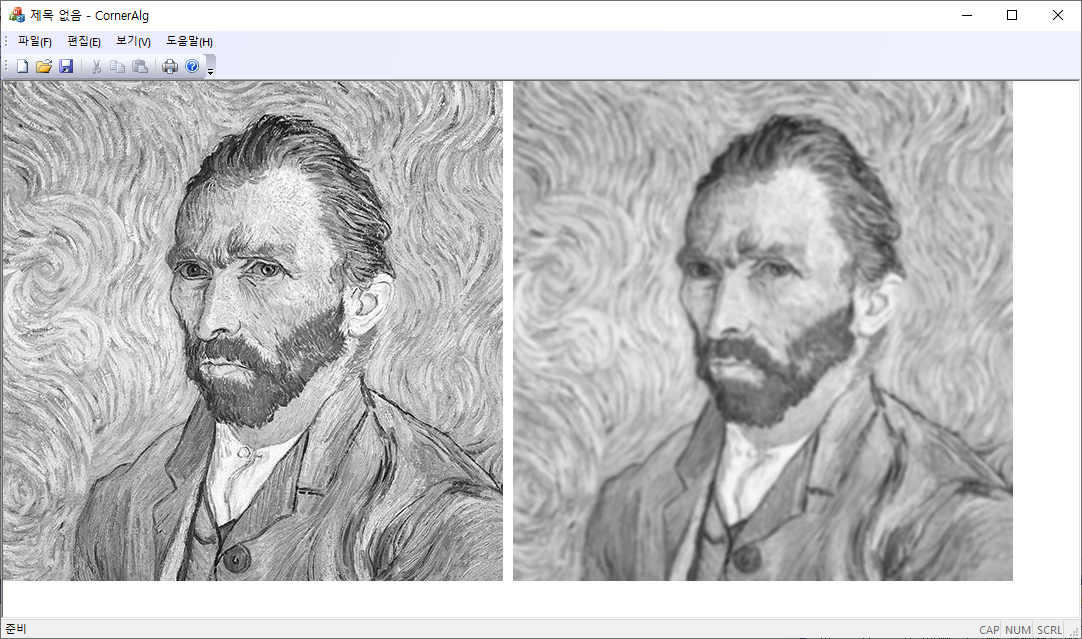
// Higher values will lead to larger regions being smoothed out.
// The sigmar value should be selected with the dynamic range of the image pixel values in mind.
// sigmas controls smoothing factor. Higher values will lead to more smoothing.
// convolution through using lookup tables.
int BilateralFilter(BYTE *image, int width, int height,
double sigmas, double sigmar, int ksize, BYTE* out) {
//const double sigmas = 1.7;
//const double sigmar = 50.;
double sigmas_sq = sigmas * sigmas;
double sigmar_sq = sigmar * sigmar;
//const int ksize = 7;
const int hksz = ksize / 2;
ksize = hksz * 2 + 1;
std::vector<double> smooth(width * height, 0);
// LUT for spatial gaussian;
std::vector<double> spaceKer(ksize * ksize, 0);
for (int j = -hksz, pos = 0; j <= hksz; j++)
for (int i = -hksz; i <= hksz; i++)
spaceKer[pos++] = exp(- 0.5 * double(i * i + j * j)/ sigmas_sq);
// LUT for image similarity gaussian;
double pixelKer[256];
for (int i = 0; i < 256; i++)
pixelKer[i] = exp(- 0.5 * double(i * i) / sigmar_sq);
for (int y = 0, imgpos = 0; y < height; y++) {
int top = y - hksz;
int bot = y + hksz;
for (int x = 0; x < width; x++) {
int left = x - hksz;
int right = x + hksz;
// convolution;
double wsum = 0;
double fsum = 0;
int refVal = image[imgpos];
for (int yy = top, kpos = 0; yy <= bot; yy++) {
for (int xx = left; xx <= right; xx++) {
// check whether the kernel rect is inside the image;
if ((yy >= 0) && (yy < height) && (xx >= 0) && (xx < width)) {
int curVal = image[yy * width + xx];
int idiff = curVal - refVal;
double weight = spaceKer[kpos] * pixelKer[abs(idiff)];
wsum += weight;
fsum += weight * curVal;
}
kpos++;
}
}
smooth[imgpos++] = fsum / wsum;
}
}
for (int k = smooth.size(); k-- > 0;) {
int a = int(smooth[k]);
out[k] = a < 0 ? 0: a > 255 ? 255: a;
}
return 1;
}728x90
'Image Recognition > Fundamental' 카테고리의 다른 글
| Cubic Spline Kernel (1) | 2024.03.12 |
|---|---|
| Ellipse Fitting (0) | 2024.03.02 |
| 파라미터 공간에서 본 최소자승 Fitting (0) | 2023.05.21 |
| 영상에 Impulse Noise 넣기 (2) | 2023.02.09 |
| Canny Edge: Non-maximal suppression (0) | 2023.01.11 |


